
# Download utils from GitHub
!wget -q --show-progress https://raw.githubusercontent.com/CLDiego/uom_fse_dl_workshop/main/colab_utils.txt -O colab_utils.txt
!wget -q --show-progress -x -nH --cut-dirs=3 -i colab_utils.txt
1. PyTorch
PyTorch is an open source machine learning and deep learning framework based on the Torch library.
Why PyTorch?
PyTorch is a popular starting point for deep learning research due to its flexibility and ease of use, compared to other frameworks like TensorFlow. It is often recommended to use TensorFlow for production-level projects, but PyTorch is a great choice for research and experimentation. More explicitly, PyTorch has the following advantages:
-
Dynamic computation graph: PyTorch uses a dynamic computation graph, which means that the graph is generated on-the-fly as operations are created. This is in contrast to TensorFlow, which uses a static computation graph. The dynamic computation graph in PyTorch makes it easier to debug and understand the code.
-
Pythonic: PyTorch is designed to be Pythonic, which means that it is easy to read and write. This is in contrast to TensorFlow, which uses a more verbose syntax.
-
Imperative programming: PyTorch uses imperative programming, which means that you can write code that looks like regular Python code. This is in contrast to TensorFlow, which uses declarative programming.
Setting up the working environment
We are going to use different python modules throughout this course. It is not necessary to be familiar with all of them at the moment. Some of these libraries enable us to work with data and perform numerical operations, while others are used for visualization purposes.
import sys
from pathlib import Path

repo_path = Path.cwd()
if str(repo_path) not in sys.path:
    sys.path.append(str(repo_path))

import utils
import pandas as pd
import torch

print("GPU available:", torch.cuda.is_available())
if torch.cuda.is_available():
    print("GPU device:", torch.cuda.get_device_name(0))
else:
    print("No GPU available. Please ensure you've enabled GPU in Runtime > Change runtime type")

checker = utils.core.ExerciseChecker("SE01")
2. Introduction to tensors
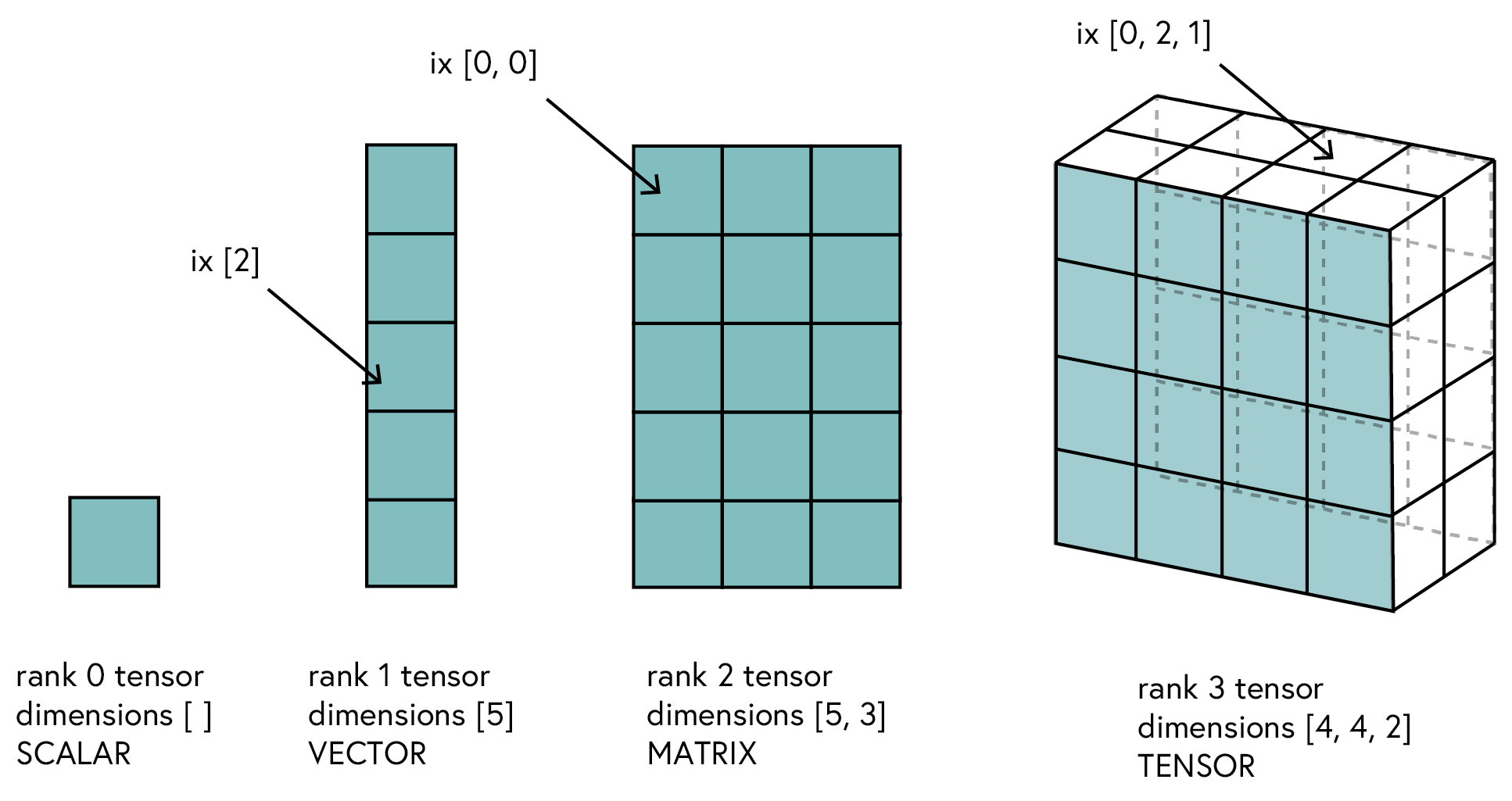
Definition: A tensor is a generalisation of vectors and matrices that can have an arbitrary number of dimensions. In simple terms, a tensor is a multidimensional array.
Similar to arrays, tensors can have different shapes and sizes. The number of dimensions of a tensor is called its rank. Here are some examples of tensors:
- Scalar: A scalar is a single number, denoted as a tensor of rank 0.
- Vector: A vector is an array of numbers, denoted as a tensor of rank 1.
- Matrix: A matrix is a 2D array of numbers, denoted as a tensor of rank 2.
- 3D tensor: A 3D tensor is a cube of numbers, denoted as a tensor of rank 3.
- nD tensor: An nD tensor is a generalisation of the above examples, denoted as a tensor of rank n.
The power of tensors comes in the form of their operations. Tensors can be added, multiplied, and manipulated in various ways.
2.1 Creating tensors
To create a tensor in PyTorch, we can use the class torch.Tensor.
Documentation: PyTorch is a well documented library, if you struggle with a function, you can always check the documentation for help. You can also use the
help()function in Python to get more information about a function or class. For example,help(torch.Tensor)will give you information about theTensorclass.
Snippet 1: Creating a scalar tensor
x = torch.tensor(101)

# Get the type and shape of the tensor
print(f'x: {x}, type: {type(x)}, shape: {x.shape}')
# Exercise 1: Creating Your First Tensor 🎯
# Try to create:
# 1. A scalar tensor with value 42
# 2. A float tensor with value 3.14

# Your code here:
scalar_tensor =  # Add your code
float_tensor = # Add your code


# ✅ Check your answer
answer = {
    'scalar_tensor': scalar_tensor,
    'float_tensor': float_tensor
}
checker.check_exercise(1, answer)
# Check the characteristics of the tensors you created
print(f"Scalar tensor: {scalar_tensor}, type: {type(scalar_tensor)}, shape: {scalar_tensor.shape}, dtype: {scalar_tensor.dtype}")
print(f"Float tensor: {float_tensor}, type: {type(float_tensor)}, shape: {float_tensor.shape}, dtype: {float_tensor.dtype}")In the above example, we created a scalar tensor with a single element. Looking at its attributes, we can see that the tensor has a shape of torch.Size([]), which means that it has no dimensions. We can also see that the tensor has a data type of torch.int64, which means that it is an integer tensor.
Note: The data type of a tensor is determined by the data type of the elements that it contains. It is important to be aware of the data type of a tensor, as it can affect the results of operations that are performed on it. Good practice is to always specify the data type of a tensor when creating it.
As we can see our single element is now stored in a type of container, which means that we can perform operations on it but not directly on the element itself. To access the element, we can use the method item().
scalar_tensor, scalar_tensor.item()We can specify the data type of a tensor by passing the dtype argument to the torch.Tensor constructor. Alternatively, we can use the ‘torch.tensor.type` method to change the data type of a tensor.
# Create a scalar tensor with a specific data type
scalar_tensor = torch.tensor(42, dtype=torch.float32)
print(scalar_tensor)

# Change the data type of a tensor
scalar_tensor = scalar_tensor.type(torch.int64)
print(scalar_tensor)

# Another way to change the data type of a tensor
scalar_tensor = scalar_tensor.int()
print(scalar_tensor)

# # Not recommended as it can be confusing
# with the .to() method that is used to move tensors
# to different devices
scalar_tensor = scalar_tensor.to(torch.float64)
print(scalar_tensor)
2.2 Initializing tensors
PyTorch provides multiple ways to initialize tensors. Sometimes, we want to create a tensor with specific values, while other times we want to create a tensor with random values. PyTorch provides several functions for creating tensors with different initializations. Below is a table summarizing some of the most commonly used tensor creation functions in PyTorch.
| Function | Description | Example | Output Shape |
|---|---|---|---|
torch.tensor() |
Creates tensor from data | torch.tensor([1, 2, 3]) |
(3,) |
torch.zeros() |
Creates tensor of zeros | torch.zeros(2, 3) |
(2, 3) |
torch.ones() |
Creates tensor of ones | torch.ones(2, 3) |
(2, 3) |
torch.rand() |
Uniform random [0, 1] | torch.rand(2, 3) |
(2, 3) |
torch.randn() |
Normal distribution μ=0, σ=1 | torch.randn(2, 3) |
(2, 3) |
torch.arange() |
Integer sequence | torch.arange(5) |
(5,) |
torch.linspace() |
Evenly spaced sequence | torch.linspace(0, 1, 5) |
(5,) |
torch.eye() |
Identity matrix | torch.eye(3) |
(3, 3) |
torch.randint() |
Random integers | torch.randint(0, 10, (2, 3)) |
(2, 3) |
# Exercise 2: Tensor Initialization 🎯
# Create the following tensors:
# 1. A 3x3 tensor of random integers between 1-10
# 2. A 3x3 identity matrix
# 3. A tensor containing evenly spaced numbers from 0 to 1 (5 numbers)
# 4. A 2x3 tensor of zeros

# Your code here:
random_tensor =  # Add your code
identity_matrix =  # Add your code
spaced_tensor =  # Add your code
zero_tensor =  # Add your code

# ✅ Check your answer
answer = {
    'random_tensor': random_tensor,
    'identity_matrix': identity_matrix,
    'spaced_tensor': spaced_tensor,
    'zero_tensor': zero_tensor
}
checker.check_exercise('2', answer)
3. Indexing tensors
Indexing tensors is similar to indexing arrays in Python. We can use square brackets [] to access elements in a tensor. This is useful for extracting specific elements or slices of a tensor. Below is a table summarizing the different ways to index tensors in PyTorch.
- Use
:to select all elements in a dimension- Use negative indices to count from the end: -1 is last element
- Ellipsis (
...) represents multiple full slices- Step values can be negative for reverse order
- Boolean masks must match tensor dimensions
| Method | Syntax | Description | Example | Result |
|---|---|---|---|---|
| Basic Indexing | tensor[ix,jx] |
Access single element | t[0,1] |
Element at row 0, col 1 |
| Slicing | tensor[start:end] |
Extract subset | t[1:3] |
Elements from index 1 to 2 |
| Striding | tensor[::step] |
Extract with step | t[::2] |
Every second element |
| Negative Indexing | tensor[-1] |
Count from end | t[-1] |
Last element |
| Boolean Indexing | tensor[mask] |
Filter with condition | t[t > 0] |
Elements > 0 |
| Ellipsis | tensor[...] |
All dimensions | t[...,0] |
All dims except last |
| Combined | tensor[1:3,...,::2] |
Mix methods | t[1:3,...,0] |
Complex selection |
# Get corners of a matrix
corners = tensor[...,[0,-1]]  # First and last elements of last dimension

# Get last row of a matrix
last_row = tensor[-1,...]  # Last row of all columns

# Extract diagonal
diagonal = tensor.diagonal()  # More efficient than indexing
# Create a 4x4 tensor for practice
practice_tensor = torch.tensor([
    [1, 2, 3, 4],
    [5, 6, 7, 8],
    [9, 10, 11, 12],
    [13, 14, 15, 16]
])

# Exercise 3: Advanced Tensor Indexing 🎯
# Extract the following from practice_tensor:
# 1. The element at position (2,3)
# 2. The second row
# 3. The last column
# 4. The 2x2 submatrix in the bottom right corner
# 5. Every even-numbered element in the first row
# 6. All corner elements as 2x2 matrix
# 7. The middle 2x2 block
# 8. The last row in reverse order

# Your code here:
position_2_3 =  # Element at (2,3)
second_row =     # Second row
last_column =   # Last column
bottom_right =  # Bottom right 2x2
even_elements =   # Even elements in first row
all_corners =   # Corner elements
middle_block =   # Middle 2x2 block

# Print results
print(f"Element at (2,3): {position_2_3}")
print(f"Second row: {second_row}")
print(f"Last column: {last_column}")
print(f"Bottom right 2x2:\n{bottom_right}")
print(f"Even elements in first row: {even_elements}")
print(f"Corner elements:\n{all_corners}")
print(f"Middle block:\n{middle_block}")


# ✅ Check your answer
answer = {
    'position_2_3': position_2_3,
    'second_row': second_row,
    'last_column': last_column,
    'bottom_right': bottom_right,
    'even_elements': even_elements,
    'all_corners': all_corners,
    'middle_block': middle_block,
}
checker.check_exercise(3, answer)
4. Tensor operations
PyTorch allows us to manipulate tensors in different ways. Since PyTorch is built on top of NumPy, the same operations can be accessed through the torch module or alternatively through the numpy module. Due to the pythonic nature of PyTorch, we can also use the same operations as we would in Python.
Basic Operations Cheatsheet
| Category | Description | Methods | PyTorch Method | Example |
|---|---|---|---|---|
| Arithmetic | Basic math operations | +, -, *, /, ** | add(), sub(), mul(), div(), pow(), sqrt() |
a + b |
| Comparison | Compare values | >, <, ==, != | gt(), lt(), eq(), ne() |
a > 0 |
| Reduction | Reduce dimensions | sum(), mean(), max() | sum(), mean(), max() |
a.sum() |
| Statistical | Statistical operations | std(), var() | std(), var() |
a.mean() |
- Type Matching: Ensure tensors have compatible data types
- Shape Broadcasting: Understand how PyTorch broadcasts shapes
- GPU Memory: Be careful with large tensor operations on GPU
- Inplace Operations: Use
_suffix for inplace operations
Common Mistakes to Avoid:
- Mixing tensor types without conversion
- Forgetting to handle device placement (CPU/GPU)
- Not checking tensor shapes before operations
- Unnecessary copying of large tensors
# Instead of: x = x + 1
x.add_(1)  # Inplace addition
y.add_(x)  # Inplace addition with another tensor
# Exercise 4: Basic Operations 🎯
# Create two 2x2 matrices:
a = torch.tensor([[1, 2], [3, 4]])
b = torch.tensor([[5, 6], [7, 8]])

# Perform the following operations:
# 1. Matrix addition (a + b)
# 2. Element-wise multiplication (a * b)
# 3. Matrix multiplication (a @ b)
# 4. Calculate square root of matrix a

# Your code here:
addition =   # Add your code
multiplication =  # Add your code
matrix_mult =   # Add your code
sqrt_a =  # Add your code

# ✅ Check your answer
answer = {
    'addition': addition,
    'multiplication': multiplication,
    'matrix_mult': matrix_mult,
    'sqrt_a': sqrt_a
}
checker.check_exercise(4, answer)
4.1 Matrix operations
Matrix multiplication is a common operation in algebra and is used in many machine learning algorithms. We can perform:
- Matrix multiplication: This is the standard matrix multiplication operation, which is denoted by the
@operator in Python. This operation is also known as the dot product. - Element-wise multiplication: This is the multiplication of two matrices of the same shape, which is denoted by the
*operator in Python. This operation is also known as the Hadamard product. - Matrix transpose: This is the operation of flipping a matrix over its diagonal, which is denoted by the
.Tattribute in Python. This operation is also known as the matrix transpose. - Matrix inverse: This is the operation of finding the inverse of a matrix, which is denoted by the
torch.inverse()function in Python. This operation is also known as the matrix inverse.
| Operation | Description | Method | Example |
|---|---|---|---|
| Matrix Multiplication | Standard matrix product | @ or matmul() | a @ b |
| Transpose | Flip matrix dimensions | .T or transpose() | a.T |
| Inverse | Matrix inverse | inverse() | torch.inverse(a) |
| Determinant | Matrix determinant | det() | torch.det(a) |
| Eigenvalues | Eigenvalues and vectors | eig() | torch.eig(a) |
| Singular Value Decomposition | SVD decomposition | svd() | torch.svd(a) |
| Cholesky Decomposition | Cholesky factorization | cholesky() | torch.cholesky(a) |
# Exercise 5: Matrix Operations 🎯
a = torch.tensor([[1, 2], [3, 4]], dtype=torch.float32)

# Perform:
# 1. Matrix multiplication with itself
# 2. Matrix transpose
# 3. Matrix determinant
# 4. Matrix inverse

matrix_mult = # Add your code
transpose =  # Add your code
determinant =  # Add your code
inverse =  # Add your code

# ✅ Check your answer
answer = {
    'matrix_mult': matrix_mult,
    'transpose': transpose,
    'determinant': determinant,
    'inverse': inverse
}
checker.check_exercise(5, answer)
4.2 Tensor Broadcasting
Since PyTorch is built on top of NumPy we can use its broadcasting capabilities. Broadcasting is how NumPy handles arrays with different shapes during arithmetic operations. It allows us to perform operations on arrays of different shapes without having to explicitly reshape them. This is done by automatically expanding the smaller array to match the shape of the larger array.
For example, if we have a 1D array of shape (3,) and a 2D array of shape (3, 2), we can add them together without having to reshape the 1D array. NumPy will automatically expand the 1D array to match the shape of the 2D array.
# Broadcasting example
a = torch.tensor([1, 2])
# Create a 2D tensor of shape (3, 2)
b = torch.tensor([[1, 2], [3, 4], [5, 6]])
# Add the two tensors together
c = a + b  # Broadcasting occurs here
print(c)  # Output: tensor([[ 2,  4], [ 4,  6], [6, 8]])
# Exercise 6: Broadcasting 🎯
# Setup tensors
matrix = torch.tensor([[1, 2], [3, 4]])
scalar = torch.tensor([2])
row = torch.tensor([1, 1])
col = torch.tensor([[2], [3]])
batch = torch.tensor([[[1, 2], [3, 4]], [[5, 6], [7, 8]]])

# Perform the following broadcasts:
# 1. Add scalar to matrix
# 2. Multiply matrix by scalar
# 3. Add row vector to matrix
# 4. Multiply matrix by column vector
# 5. Scale batch by scalar

# Your code here:
broadcast_add = # Add your code
broadcast_mult =  # Add your code
row_add =  # Add your code
col_mult =  # Add your code
batch_scale =  # Add your code

# Print results to understand broadcasting
print(f"Original matrix shape: {matrix.shape}")
print(f"After scalar addition: {broadcast_add.shape}")
print(f"After row broadcast: {row_add.shape}")
print(f"After column broadcast: {col_mult.shape}")
print(f"After batch scaling: {batch_scale.shape}")

# ✅ Check your answer
answer = {
    'broadcast_add': broadcast_add,
    'broadcast_mult': broadcast_mult,
    'row_add': row_add,
    'col_mult': col_mult,
    'batch_scale': batch_scale
}
checker.check_exercise(6, answer)
4.3 Reshaping Methods
Sometimes, we need to change the shape of a tensor without changing its data. We do this in order to prepare the tensor for a specific operation or to match the shape of another tensor. PyTorch provides several methods for reshaping tensors. Below is a table summarizing some of the most commonly used reshaping methods in PyTorch.
| Method | Description | Example | Note |
|---|---|---|---|
reshape() |
New shape, maybe new memory | x.reshape(2,3) |
May copy data |
view() |
New shape, same memory | x.view(2,3) |
Must be contiguous |
squeeze() |
Remove single dims | x.squeeze() |
Removes size 1 dims |
unsqueeze() |
Add single dim | x.unsqueeze(0) |
Adds size 1 dim |
expand() |
Broadcast dimensions | x.expand(2,3) |
No data copy |
# Create a 1D tensor of shape (6,)
x = torch.tensor([1, 2, 3, 4, 5, 6])
# Reshape to (2, 3)
print(x.reshape(2, 3))  # Output: tensor([[1, 2, 3], [4, 5, 6]])
# Exercise 7: Reshaping 🎯
# Setup tensors
flat = torch.tensor([1, 2, 3, 4, 5, 6])
ones = torch.ones(1)
vector = torch.tensor([1, 2, 3])

# Perform:
# 1. Reshape flat tensor to (3,2) matrix
# 2. Expand ones to (3,1) matrix
# 3. Reshape vector to be broadcastable with (3,3) matrix

reshaped =  # Add your code
expanded =  # Add your code
broadcast_ready =   # Add your code

# Verify broadcasting works
test_matrix = torch.ones(3, 3)
result = test_matrix * broadcast_ready
print(f"Broadcast result shape: {result.shape}")

# ✅ Check your answer
answer = {
    'reshaped': reshaped,
    'expanded': expanded,
    'broadcast_ready': broadcast_ready
}
checker.check_exercise(7, answer)
5. Automatic Differentiation (Autograd)
Automatic differentiation is one of the most powerful features of PyTorch. It allows us to compute gradients automatically, which is essential for training neural networks. PyTorch uses a technique called reverse mode differentiation to compute gradients efficiently. This technique is based on the chain rule of calculus and allows us to compute gradients for complex functions with many variables.
requires_grad=True.
Take for instance the following function:
\[f(x) = x^2 + 42y^2 + 3\]where $x$ and $y$ are tensors. The gradient of this function with respect to $x$ and $y$ is given by:
\[\frac{\partial f}{\partial x} = 2x\] \[\frac{\partial f}{\partial y} = 84y\]using the chain rule of calculus. PyTorch allows us to compute these gradients automatically using the backward() method.
The chain rule is a fundamental concept in calculus that allows us to compute the derivative of a composite function. It states that if we have two functions $f(x)$ and $g(x)$, then the derivative of their composition $f(g(x))$ is given by:
\[\frac{d}{dx}f(g(x)) = f'(g(x)) \cdot g'(x)\]where $f’(g(x))$ is the derivative of $f$ with respect to $g$, and $g’(x)$ is the derivative of $g$ with respect to $x$. This means that we can compute the derivative of a composite function by computing the derivatives of its constituent functions and multiplying them together.
5.1 Autograd Concepts
In PyTorch, the autograd engine keeps track of all operations performed on tensors with requires_grad=True. It builds a computation graph dynamically as operations are performed. This graph is used to compute gradients when we call the backward() method.
| Concept | Description | Example |
|---|---|---|
requires_grad |
Flag to track gradients | x = torch.tensor(1.0, requires_grad=True) |
backward() |
Compute gradients | y.backward() |
grad |
Access gradients | x.grad |
# Create tensor with gradient tracking
x = torch.tensor([1.0], requires_grad=True)

# Compute function
y = x * x

# Compute gradient
y.backward()

# Access gradient
x.grad  # Should be 2.0
# Exercise 8: Autograd 🎯
x = torch.tensor([2.0], requires_grad=True)

# Compute y = 3x^3 + 2x^2 - 5x + 1
# Derivative at x=2 should be 3(3x^2) + 2(2x) - 5 = 3(12) + 2(4) - 5 = 36 + 8 - 5 = 39

y =  # Add your code

# Compute the gradient
# Add your code

# Print the gradient
print(f"Gradient at x=2: {x.grad}")

# ✅ Check your answer
answer = {
    'grad_value': x.grad,
    'requires_grad': x.requires_grad
}
checker.check_exercise(8, answer)
6. Data to tensors
As mentioned before, PyTorch inherent pythonic nature allows us to easily convert existing data structures to tensors. Thus, we can use different data science libraries to load data and convert it to tensors. We are going to use the pandas library to load data from CSV files and convert it to tensors.
First, let’s download the data. We will be using the ARKOMA dataset. We will explore the dataset in the next section. For now, we will just download it and load it into a pandas dataframe.
data_path = Path(Path.cwd(), 'datasets')
dataset_path = utils.data.download_dataset('ARKOMA',
                                   dest_path=data_path,
                                   extract=True)

dataset_path = dataset_path / 'Left Arm Dataset' / 'LTrain_x.csv'
6.1 Loading data with pandas
DataFrames in pandas are similar to tables in SQL or Excel. They are two-dimensional data structures that can hold different types of data. DataFrames have rows and columns, where each column can have a different data type. We can use the pandas library to load data from CSV files and convert it to DataFrames.
# Read the dataset
df = pd.read_csv(dataset_path)

# Display the statistics of the dataset
df.describe().T
# Get the data as a numpy array
type(df.Px.values)To pass the data to PyTorch, we need to convert the DataFrame to a NumPy array and then to a tensor. We can do this using the values attribute of the DataFrame and the torch.tensor() function.
***
col_val = df['column_name'].values  # Get column values as NumPy array
tensor = torch.tensor(col_val)  # Convert to tensor
# Exercise 9: Pandas to Tensors 🎯
# Given the DataFrame df with NAO robot arm data
# Perform the following:
# 1. Convert the 'Px' column to a tensor
# 2. Convert the 'Py' column to a tensor
# 3. Create a tensor from all position columns (Px, Py, Pz)
# 4. Create a tensor of all columns and convert to float32

# Your code here:
px_tensor = # Add your code
py_tensor =  # Add your code
pos_tensor =  # Add your code
all_data =  # Add your code

# Print shapes
print(f"px_tensor shape: {px_tensor.shape}")
print(f"py_tensor shape: {py_tensor.shape}")
print(f"pos_tensor shape: {pos_tensor.shape}")
print(f"all_data shape: {all_data.shape}")

# ✅ Check your answer
answer = {
    'px_tensor': px_tensor,
    'py_tensor': py_tensor,
    'pos_tensor': pos_tensor,
    'all_data': all_data
}
checker.check_exercise(9, answer)
7. Using the GPU
PyTorch allows us to use the GPU to accelerate computations. This is done by moving the tensors to the GPU memory. We can do this by using the to method of a tensor and passing the device as an argument. The device can be either cuda or cpu. The cuda device refers to the GPU, while the cpu device refers to the CPU.
# Check if GPU is available
if torch.cuda.is_available():
    device = torch.device('cuda')  # Use GPU
else:
    device = torch.device('cpu')  # Use CPU
# Check GPU availability
device = torch.device("cuda" if torch.cuda.is_available() else "cpu")

print(f"Device: {device}")

# Move the tensor to the GPU
px_tensor = px_tensor.to(device)
print(f'Tensor moved to device: {px_tensor.device}')
torch.device()function. The device ID is a number that identifies the GPU. For example, if we have two GPUs, we can use the first GPU by specifyingcuda:0and the second GPU by specifyingcuda:1. We can also use thetorch.cuda.device_count()function to get the number of available GPUs.
7.1 When to use the GPU
Using the GPU is beneficial when we are working with large tensors or when we are performing operations that are computationally expensive. For example, training a deep learning model on a large dataset can be accelerated by using the GPU. However, if we are working with small tensors or performing simple operations, using the CPU may be faster.
Typically, we use the GPU for computer vision and natural language processing tasks, where the data is large and the operations are computationally expensive.
Note: When choosing between the CPU and GPU, it is important to make sure that all tensors and models are on the same device. If a tensor is on the CPU and a model is on the GPU, PyTorch will automatically move the tensor to the GPU, which can lead to performance issues. It is important to be aware of which device each tensor and model is on.