
# Download utils from GitHub
!wget -q --show-progress https://raw.githubusercontent.com/CLDiego/uom_fse_dl_workshop/main/colab_utils.txt -O colab_utils.txt
!wget -q --show-progress -x -nH --cut-dirs=3 -i colab_utils.txt
from pathlib import Path
import sys
repo_path = Path.cwd()
if str(repo_path) not in sys.path:
sys.path.append(str(repo_path))
import utils
from tqdm import tqdm
from sklearn.model_selection import train_test_split
import matplotlib.pyplot as plt
import pandas as pd
import torch
print("GPU available:", torch.cuda.is_available())
if torch.cuda.is_available():
print("GPU device:", torch.cuda.get_device_name(0))
else:
print("No GPU available. Please ensure you've enabled GPU in Runtime > Change runtime type")
challenger_temp = 0.56
checker = utils.core.ExerciseChecker("SE02")1. Artificial Neural Networks
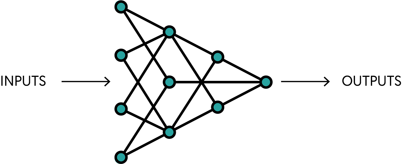
Artificial Neural Networks (ANNs) are machine learning models inspired by the human brain, consisting of interconnected nodes (neurons) organized in layers. They form the foundation of deep learning and typically contain:
- Input layer: Receives the initial data/features
- Hidden layer(s): Processes the information
- Output layer: Produces the final prediction/result
Each neuron connects to neurons in the next layer through weighted connections that are adjusted during training to minimize the difference between predicted and actual outputs.
1.1 Neurons
Definition: Neurons are the basic building blocks of ANNs, similar to biological neurons. Each neuron receives inputs, applies a transformation, and produces an output.
The basic structure of a neuron can be seen below:
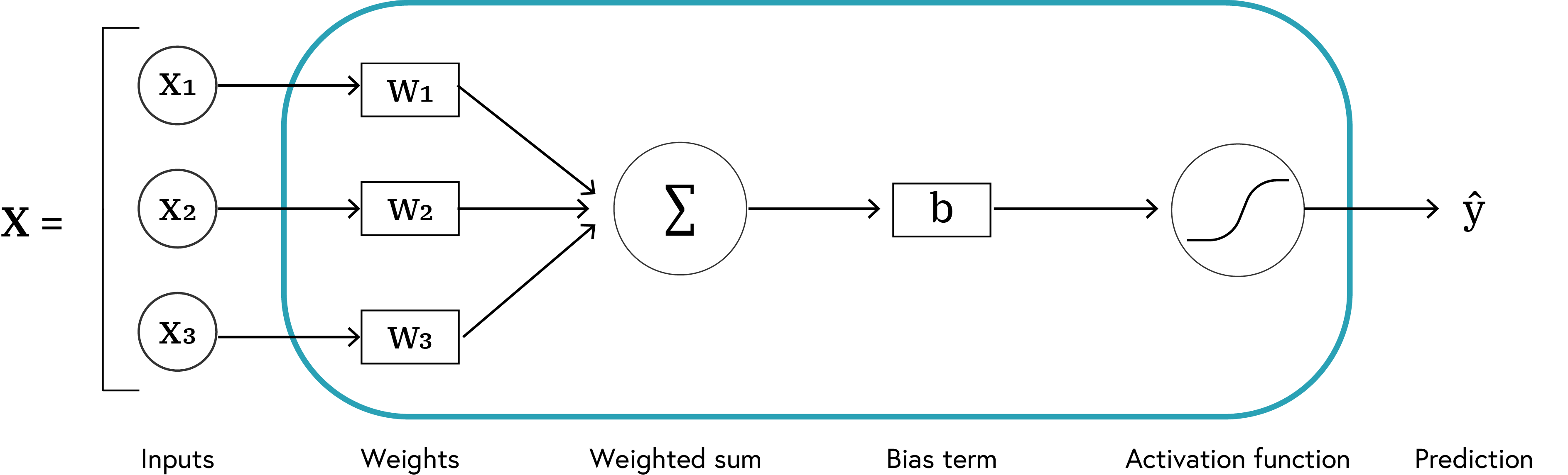
Neuron Output Formula
The output of a neuron after applying the activation function is: \(\hat{y} = f(W \cdot X + b)\)
where:
- $ \hat{y} $ Predicted output of the neuron (may differ from actual output)
- $ f $ Activation function (introduces non-linearity, e.g., sigmoid, tanh, ReLU)
- $ W $ Weight vector (determines connection strengths)
- $ X $ Input vector (features of the data)
- $ b $ Bias term (shifts the activation function)
- $ \cdot $ Dot product between weight and input vectors
1.1.1 Features and Targets
In neural networks:
- Features (X): Input variables/attributes used for prediction
- Targets (y): Values we’re trying to predict (ground truth labels)
Now let’s implement a neuron in Python using PyTorch. We’ll create a Neuron class that handles the forward pass - passing inputs to the neuron and computing the output.
Note: We’ll use PyTorch’s
torch.nn.Moduleas a base class andtorch.nn.Parameterto define weights and biases, making them learnable parameters that can be updated during training.
Snippet 1: nn.Module and nn.Parameter
weight = torch.nn.Parameter(torch.randn(2, 1), requires_grad=True)
bias = torch.nn.Parameter(torch.randn(1))
# Exercise 1: Implementing a Neuron 🎯
# Implement:
# 1. The sigmoid function
# 2. A neuron using torch.nn.Module but with manual parameter handling
# 3. Create a neuron with specified input features and initialize weights
# 4. Define an input vector x with two features
# 5. Use the neuron to compute an output

def sigmoid(x:torch.Tensor) -> torch.Tensor:
    # The sigmoid function is defined as:
    # sigmoid(x) = 1 / (1 + exp(-x))
    return # Add your code

class Perceptron(torch.nn.Module):
    def __init__(self, n_features:int, activation:callable=sigmoid) -> None:
        # Initialize the neuron as a PyTorch module
        super().__init__()
        # Initialize weights with random values - Parameter makes it learnable
        self.weights = # Add your code

        # Initialize bias to a random value
        self.bias = # Add your code

        self.activation = # Add your code


    def forward(self, x:torch.Tensor) -> torch.Tensor:
        # 1. Compute linear output manually (dot product of inputs and weights + bias)
        # 2. Apply the activation function to the result
        # 3. Return the output

        linear_output = # Add your code

        output = # Add your code

        return output

    def __repr__(self) -> str:
        """String representation of the neuron"""
        return f"Neuron (weights = {self.weights.detach()}, bias = {self.bias.detach()})"

# Create a neuron with 2 input features
neuron = Perceptron(n_features=2)

# Define an input vector x with two features
# with values 1.0, 2.0
x = # Add your code

# Let's use our neuron to compute an output
output = neuron(x)  # In PyTorch modules, we call the object directly instead of .forward()

# Print the output to see the result
print(f"Output from neuron: {output.item()}")
print(neuron)
print(f"Neuron has {len(neuron.weights)} weights")

# ✅ Check your answer
answer = {
    'sigmoid': sigmoid,
    'neuron_output': output,
    'neuron_input_size': len(neuron.weights),
    'has_bias': hasattr(neuron, 'bias'),
    'is_parameterized': isinstance(neuron.weights, torch.nn.Parameter)
}
checker.check_exercise(1, answer)
fig, ax, G, pos = utils.plotting.visualize_network_nx(neuron, figsize=(16, 4))
# Display information about the perceptron
print(f"Perceptron Architecture:")
print(f" - Input features: {len(neuron.weights)}")
print(f" - Activation function: {neuron.activation.__name__ if hasattr(neuron.activation, '__name__') else 'Custom'}")
print(f" - Output: 1 (probability between 0 and 1)")
print(f"\nGraph Properties:")
print(f" - Number of nodes: {G.number_of_nodes()}")
print(f" - Number of edges: {G.number_of_edges()}")2. Using Neurons to Solve Problems
Case Study: Space Shuttle Challenger Disaster
The explosion of the Space Shuttle Challenger on January 28, 1986, resulted from the failure of O-rings sealing the propulsion system. Critical components hadn’t been properly tested at low temperatures, leading to catastrophic failure.
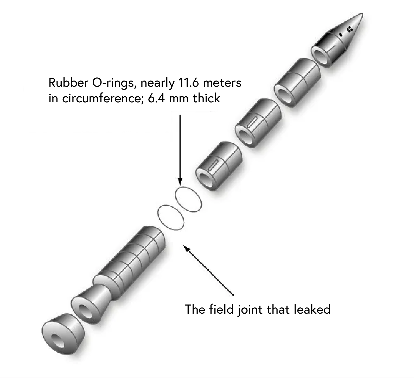
We’ll analyze data from the Challenger disaster, examining the relationship between temperature at launch and O-ring failures. This real-world example demonstrates how neural networks can identify crucial patterns that might prevent disasters.
Dataset Description
| Variable | Description |
|---|---|
n_risky |
Number of O-rings at risk during launch |
n_distressed |
Number of O-rings experiencing thermal distress |
temp |
Temperature at launch (in degrees Fahrenheit) |
leak_psi |
Pressure at which the O-rings leak |
temporal_order |
Temporal order of the launch |
data_path = Path(Path.cwd(), 'datasets')
dataset_path = utils.data.download_dataset('challenger',
                                           dest_path=data_path,
                                           extract=True,
                                           remove_compressed=True)
dataset_path = dataset_path / 'o-ring-erosion-only.data'
cols = ['n_risky', 'n_distressed', 'temp', 'leak_psi', 'temporal_order']
df = pd.read_csv(dataset_path, sep="\\s+", header=None, names=cols)
df.describe().T2.1 Preparing the Data
We’ll build a model that predicts launch success based on temperature. Our goal is to use the temp variable as a feature to predict the n_distressed variable (O-ring failures).
Pre-processing Steps
- Convert temperature from Fahrenheit to Celsius
- Cap the number of distressed O-rings to be between 0 and 1 (binary outcome)
- Normalize the temperature using standardization (z-score)
- Split the data into training and test sets
.view(-1, 1)for reshaping in PyTorch.
from sklearn.model_selection import train_test_split

X_train, X_test, y_train, y_test = train_test_split(X, y, test_size=0.2, random_state=42)
# Exercise 2: Data Preparation 🎯
# Implement:
# 1. Convert temperature from Fahrenheit to Celsius
# 2. Cap n_distressed values at 1.0 (binary outcome)
# 3. Convert features and targets to PyTorch tensors
# 4. Normalize the temperature data
# 5. Split the data into training and testing sets (80% train, 20% test)

# Step 1: Convert temperature from Fahrenheit to Celsius
def f_to_c(f:float) -> float:
    # The conversion formula is:
    # C = (F - 32) * 5 / 9
    return # Add your code

# Apply the conversion function to the temperature column
temp = # Add your code

# Step 2: Cap the n_distressed at 1.0 (binary outcome)
n_distressed = # Add your code

# Step 3: Convert features and targets to PyTorch tensors
X = # Add your code
y = # Add your code

# Step 4: Normalize the temperature data for better training
# Use Standardization (z-score normalization)
X_mean = # Add your code
X_std = # Add your code
X_normalized = # Add your code

# Step 5: Split the data into training and testing sets (80% train, 20% test)
X_train, X_test, y_train, y_test = # Add your code
# Print the shapes of the training and testing sets
print(f"Training data shape: {X_train.shape} inputs and {y_train.shape} targets")
print(f"Testing data shape: {X_test.shape} inputs and {y_test.shape} targets")
print(f"Temperature mean: {X_mean.item():.2f}°C, std: {X_std.item():.2f}°C")
print(f"Number of O-ring distress cases: {y.sum().item()} out of {len(y)}")
print(f"Number of O-ring distress cases: {y.sum().item()} out of {len(y)}")

# ✅ Check your answer
answer = {
    'f_to_c': f_to_c,
    'X_shape': X_normalized.shape,
    'y_shape': y.shape,
    'X_mean': X_mean.item(),
    'X_std': X_std.item(),
    'n_distress_cases': y.sum().item(),
    'data_clipped': bool(n_distressed.max() <= 1.0),
    'train_test_split_ratio': len(X_train) / len(X) >= 0.75 and len(X_train) / len(X) <= 0.85,
    'tensors_created': isinstance(X, torch.Tensor) and isinstance(y, torch.Tensor)
}

checker.check_exercise(2, answer)

# Plot the data to visualize the relationship
fig, ax = plt.subplots(figsize=(12, 4))
ax.scatter(X.numpy(), y.numpy(), alpha=0.5, edgecolors='k')

utils.plotting.make_fig_pretty(ax, title="O-Ring Distress vs Temperature",
                             xlabel="Temperature (°C)", ylabel="Distress")
2.2 The Forward Pass
In our O-ring example:
- Feature: Temperature (X_normalized) - what our model uses for predictions
- Target: O-ring distress (y) - what we’re trying to predict
Forward Pass Process
| Step | Description |
|---|---|
| 1 | Input data (features) is fed into the network |
| 2 | Each layer processes the inputs it receives |
| 3 | Activation functions add non-linearity |
| 4 | Final layer produces output predictions |
For our single neuron model with temperature as input, this is expressed as:
\[\hat{y} = \sigma(w \cdot \text{temperature} + b)\]2.2.1 Batch Processing vs. Individual Samples
In our implementation, we’re processing one sample at a time in our loops:
for i in range(len(X_normalized)):
    predictions[i] = model(X_normalized[i])
This approach works for our small dataset (23 samples) and single feature, but in production machine learning, data is typically processed in batches for efficiency:
# Process all samples in a single operation
predictions = model(X_normalized)  # For batch-compatible models
2.3 Loss Functions and Error Measurement
Why Measure Error?
Loss functions provide quantitative feedback on model performance:
- Optimization guidance: Indicates direction for weight/bias adjustments
- Performance tracking: Monitors model improvement during training
- Model comparison: Provides objective metrics for different models
- Convergence detection: Helps determine when to stop training
Mean Squared Error (MSE)
We’ll use the MSE loss function, defined as: \(\text{MSE} = \frac{1}{n} \sum_{i=1}^{n} (y_i - \hat{y}_i)^2\)
Where:
- $ n $ number of samples
- $ y_i $ actual target value for sample $ i $
- $ \hat{y}_i $ predicted target value for sample $ i $
# Exercise 3: Implementing a Loss Function 🎯
# In this exercise, you will:
# 1. Implement a Mean Squared Error (MSE) loss function
# 2. Create a modified neuron for the O-ring data
# 3. Compute predictions using the forward pass
# 4. Calculate the loss between predictions and actual targets

def mse_loss(predictions: torch.Tensor, targets: torch.Tensor) -> torch.Tensor:
    """Mean Squared Error loss function

    MSE = 1/n * Σ (predictions - targets)²
    where n is the number of samples.
    """
    # Calculate the squared difference between predictions and targets
    squared_diff = # Add your code

    # Return the mean of the squared differences
    return # Add your code

# Create a neuron specifically for the temperature data (1 input feature)
model = # Add your code
print(f"Initial model: {model}")

# Forward pass: Feed the normalized temperature data through the neuron
predictions = torch.zeros_like(y)

# Loop through each input sample and compute the prediction
for i in tqdm(range(len(X_normalized)), desc="Computing predictions"):
    # Use the model to compute the prediction for each input sample
    predictions[i] = # Add your code


# Calculate the loss using our MSE loss function
loss = mse_loss(predictions, y)
print(f"Initial loss: {loss.item():.4f}")

# Alternatively, we can use PyTorch's built-in MSE loss function
pytorch_mse = torch.nn.MSELoss()
loss_pytorch = pytorch_mse(predictions, y)
print(f"PyTorch MSE loss: {loss_pytorch.item():.4f}")

# Check if our implementation matches PyTorch's (should be very close)
loss_function_correct = torch.isclose(loss, loss_pytorch, rtol=1e-4)
print(f"Our MSE implementation matches PyTorch: {loss_function_correct}")

# ✅ Check your answer
answer = {
    'mse_loss': mse_loss,
}
checker.check_exercise(3, answer)
2.4 The Backward Pass (Backpropagation)
After computing the loss, we need to adjust our model’s parameters (weights and bias) to improve predictions. This is done through backpropagation.
Backpropagation Process
| Step | Description | |
|---|---|---|
| 1 | Computing gradients | Calculate how loss changes with respect to each parameter |
| 2 | Propagating error backward | Work from output layer back to input layer |
| 3 | Applying the chain rule | Break down complex derivatives into simpler parts |
Gradient Descent Update Rule
Once we have gradients, we update parameters:
\(w_{new} = w_{old} - \alpha \frac{\partial L}{\partial w}\) \(b_{new} = b_{old} - \alpha \frac{\partial L}{\partial b}\)
Where:
- $\alpha$ learning rate (controls step size)
- $\frac{\partial L}{\partial w}$ gradient of loss with respect to weight
- $\frac{\partial L}{\partial b}$ gradient of loss with respect to bias
PyTorch’s Autograd System
When requires_grad=True is set on tensors (default for nn.Parameter):
- PyTorch tracks operations in a computational graph
- When we call
loss.backward(), PyTorch computes gradients for all tracked tensors - Gradients are stored in the
.gradattribute of each tensor - Gradients should be zeroed out before each training iteration to avoid accumulation from previous iterations. For the parameters, we can use
parameter.grad.zero_()to reset gradients.
Neural Network Training Cycle
| Phase | Description |
|---|---|
| Forward Pass | Compute predictions with current parameters |
| Loss Calculation | Measure error between predictions and true values |
| Backward Pass | Compute gradients of loss with respect to parameters |
| Parameter Update | Adjust parameters to reduce loss |
This cycle repeats for multiple epochs until the model converges to a solution.
Now let’s implement the backward pass and parameter updates for our O-ring prediction model.
# Exercise 4: Implementing the Backward Pass and Parameter Updates 🎯
# In this exercise, you will:
# 1. Implement a training loop with forward and backward passes
# 2. Use PyTorch's autograd to compute gradients
# 3. Update the model parameters using gradient descent
# 4. Visualize how the model's predictions improve over time

# Reset our model for training
model = Perceptron(n_features=1)
print(f"Initial model parameters: {model}")

# Define training hyperparameters
learning_rate = # Add your code
num_epochs = # Add your code

# Lists to store training progress
train_losses = []

# Training loop
for epoch in tqdm(range(num_epochs), desc="Training Progress", bar_format="{desc}: {percentage:3.0f}%|{bar}| {n_fmt}/{total_fmt} [Time: {elapsed}<{remaining}]"):
    # Forward pass: compute predictions
    predictions = torch.zeros_like(y)
    for i in range(len(X_normalized)):
        predictions[i] = # Add your code

    # Compute loss
    loss = # Add your code
    train_losses.append(loss.item())

    # Backward pass: compute gradients
    # Add your code

    # Update parameters using gradient descent
    with torch.no_grad():  # No need to track gradients during the update
        # Your code here: Update weights using gradient descent
        model.weights -= # Add your code
        # Your code here: Update bias using gradient descent
        model.bias -= # Add your code

    # Zero gradients for the next iteration
    # Your code here: Zero out the gradients
    # Add your code
    # Add your code

print(f"Final model parameters: {model}")
print(f"Final loss: {train_losses[-1]:.4f}")

# Calculate final predictions
with torch.no_grad():
    final_predictions = torch.zeros_like(y)
    for i in range(len(X_normalized)):
        final_predictions[i] = model(X_normalized[i])

# ✅ Check your answer - is the loss decreasing over time?
answer = {
    'training_convergence': train_losses[0] > train_losses[-1],
    'final_loss': train_losses[-1],
    'negative_weight': model.weights.item() < 0
}
checker.check_exercise(4, answer)
# Create a figure with two subplots side by side
fig, (ax1, ax2) = plt.subplots(1, 2, figsize=(20, 6))
# Plot training loss
utils.plotting.plot_loss(
train_losses,
title="Training Loss Over Time",
tufte_style=True,
title_fsize=18,
ax=ax1
)
# Plot model predictions
utils.plotting.plot_model_predictions_SE02(
model=model,
X=X_normalized,
y=y,
X_mean=X_mean.item(),
X_std=X_std.item(),
special_temp=challenger_temp,
special_temp_label=f'Challenger Launch: {challenger_temp:.1f}°C',
title="O-Ring Failure Probability vs Temperature",
tufte_style=True,
ax=ax2,
title_fsize=18,
)
plt.tight_layout()
plt.show()# Interactive visualization of the O-ring failure model
# This uses our external interactive visualization function
# Create the interactive visualization widget
main_ui, out = utils.plotting.create_interactive_neuron_visualizer(
X=X_normalized,
y=y,
X_mean=X_mean.item(),
X_std=X_std.item(),
challenger_temp=challenger_temp,
neuron_class=Perceptron,
loss_function=mse_loss,
initial_weight=float(model.weights.item()),
initial_bias=float(model.bias.item()),
learning_rate=0.1,
training_epochs=100
)
# Display the interactive widget
display(main_ui, out)2.5 Using the model to predict O-ring distress
Having trained out model, we now want to use it to predict the potential for O-ring distress at different temperatures. Using models in this way is called inference. To do this, we need to consider the following:
- Data preparation: The data we want to predict on needs to be in the same format as the data we trained on. This means that we need to apply the same transformations (e.g., normalization) to the new data.
- Gradient tracking: When we are using the model for inference, we do not need to track gradients. This is because we are not updating the model parameters during inference. We can use
torch.no_grad()to disable gradient tracking. - Model input: The model input should be a tensor with the same shape as the training data. If we are predicting on a single sample, we need to add an extra dimension to the tensor to make it 2D.
Let’s implement the inference process for our O-ring prediction model.
# Exercise 5: Making Predictions for the Challenger Launch 🎯
# In this exercise, you will make predictions about the O-ring failure at the Challenger launch temperature
# and calculate the relative risk compared to normal temperatures

# The Challenger launch temperature was 31°F (-0.56°C)
challenger_launch_temp = f_to_c(31.0)
print(f"Challenger launch temperature: {challenger_launch_temp:.2f}°C")

# Normalize the temperature using the same parameters as our training data
challenger_temp_normalized = # Add your code
challenger_tensor = # Add your code

# Use the trained model to predict the probability of O-ring failure
with torch.no_grad():
    failure_probability = model(challenger_tensor).item()

print(f"Predicted probability of O-ring failure: {failure_probability:.4f} or {failure_probability*100:.1f}%")

# Determine if this probability indicates a high risk
# A common threshold in binary classification is 0.5 (50% probability)
failure_risk = "HIGH RISK" if failure_probability > 0.5 else "LOW RISK"

# What is your launch recommendation based on this analysis?
launch_recommendation = "DO NOT LAUNCH" if failure_probability > 0.5 else "PROCEED WITH LAUNCH"

print(f"Risk assessment: {failure_risk}")
print(f"Launch recommendation: {launch_recommendation}")

# Calculate how many times more likely failure is at the launch temperature compared to a warmer day (20°C)
warm_temp = 20.0  # A much warmer temperature in Celsius
warm_temp_normalized = (warm_temp - X_mean.item()) / X_std.item()
warm_tensor = torch.tensor([warm_temp_normalized], dtype=torch.float32)

with torch.no_grad():
    warm_failure_probability = model(warm_tensor).item()

relative_risk = failure_probability / warm_failure_probability if warm_failure_probability > 0 else float('inf')
print('-' * 80)
print(f"Probability of failure at 20°C: {warm_failure_probability:.4f} or {warm_failure_probability*100:.1f}%")
print(f"Failure at launch temperature is {relative_risk:.1f}x more likely than at 20°C")


# ✅ Check your answer
answer = {
    'challenger_failure_prob': failure_probability,
    'recommendation': launch_recommendation == "DO NOT LAUNCH",
    'relative_risk_factor': relative_risk > 3,  # Is risk at least 3 times higher?
}
checker.check_exercise(5, answer)
2.6 Key Insights from Our Analysis
Our trained model shows a strong correlation between temperature and O-ring failure probability. At the Challenger launch temperature of 31°F (-0.56°C), the model predicts an extremely high probability of failure.
Critical Lessons
| Insight | Description |
|---|---|
| Temperature threshold | Risk increases dramatically below a critical temperature point |
| Data-driven decisions | Statistical analysis could have provided strong evidence against launching |
| Risk assessment | The model correctly identifies risk despite limited low-temperature data |
| Communication | Technical findings must be effectively communicated to decision-makers |
The Rogers Commission, which investigated the disaster, found that NASA managers had disregarded warnings from engineers about the dangers of launching in cold temperatures—a tragic example of how crucial effective communication of technical risks can be.
2.6.1 The Challenger Disaster and Data Science Ethics
Our analysis demonstrates a sobering point: proper data analysis could have potentially prevented this disaster. As our model shows, the probability of O-ring failure increases dramatically at lower temperatures, and the launch temperature of 31°F (-0.56°C) was well within the danger zone.