# Download utils from GitHub
!wget -q --show-progress https://raw.githubusercontent.com/CLDiego/uom_fse_dl_workshop/main/colab_utils.txt -O colab_utils.txt
!wget -q --show-progress -x -nH --cut-dirs=3 -i colab_utils.txt

from pathlib import Path
import sys

repo_path = Path.cwd()
if str(repo_path) not in sys.path:
    sys.path.append(str(repo_path))


import utils 
import shutil
import requests
import random
import torch
import numpy as np
import matplotlib.pyplot as plt
from io import BytesIO
from PIL import Image

torch.manual_seed(42)
torch.cuda.manual_seed(42)
random.seed(42)
torch.backends.cudnn.deterministic = True
torch.backends.cudnn.benchmark = False

print("GPU available:", torch.cuda.is_available())
if torch.cuda.is_available():
    print("GPU device:", torch.cuda.get_device_name(0))
else:
    print("No GPU available. Please ensure you've enabled GPU in Runtime > Change runtime type")

ascent_url = 'https://raw.githubusercontent.com/CLDiego/uom_fse_dl_workshop/main/figs/ascent.jpg'
response = requests.get(ascent_url)
response.raise_for_status() 
checker = utils.core.ExerciseChecker("SE04")

1. Convolutional Neural Networks (CNNs)

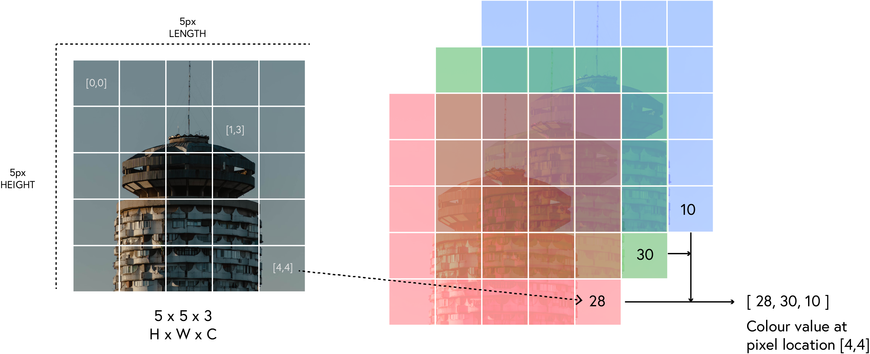
Definition: Convolutional Neural Networks (CNNs) are a specialized type of neural network designed for processing structured grid-like data, such as images, by using mathematical operations called convolutions.

CNNs have revolutionized computer vision tasks and are the foundation of many modern systems for image recognition, object detection, segmentation, and more. Their architecture is inspired by the organization of the visual cortex in animals, where individual neurons respond to stimuli in restricted regions called receptive fields.

1.1 Why Standard Neural Networks Struggle with Images

Images present unique challenges that make standard fully-connected neural networks inefficient:

Challenge	Description
Spatial Relationships	Standard networks don’t account for spatial relationships between pixels
Parameter Explosion	A 224×224×3 image would require over 150,000 weights per neuron
Translation Invariance	Objects can appear anywhere in an image but have the same meaning
Feature Hierarchy	Images contain low-level features (edges, textures) that compose into higher-level features

CNNs address these challenges through specialized architecture components that we’ll explore in this workshop.

Let’s begin by understanding the core operation that gives CNNs their name: convolution.

2. The Convolution Operation

Definition: A convolution in the context of CNNs is a mathematical operation that combines two functions by multiplying them and integrating over their overlapping regions.

In simple terms, convolution involves sliding a small window (called a filter or kernel) over an image and performing an element-wise multiplication between the filter and the pixel values, then summing the results to produce a single output value for each position.

2.1 How Convolution Works

Step	Description
1	Position the filter at the top-left corner of the image
2	Perform element-wise multiplication between the filter and the corresponding image pixels
3	Sum all the resulting values to get a single output value
4	Move the filter to the next position (typically one pixel to the right)
5	Repeat steps 2-4 until the entire image has been covered

This process creates what’s called a feature map, which highlights specific patterns or features in the image that match the filter pattern.

Note: In deep learning libraries, what’s actually implemented is technically cross-correlation rather than convolution (the filter is not flipped). However, since the filters are learned during training, this distinction doesn’t matter in practice.

Let’s first load an example image to work with:

asc_image = Image.open(BytesIO(response.content)).resize((256, 256))
asc_image

2.2 Key Parameters in Convolution

The convolution operation is governed by several key parameters that affect the output dimensions and characteristics of the feature map. PyTorch provides a convenient way to implement convolutional layers using the torch.nn.Conv2d class. The key parameters include:

Parameter	Description	Effect on Output Dimensions
Kernel Size	The dimensions of the filter (e.g., 3×3, 5×5)	Larger kernels reduce output size more
Stride	How many pixels the filter shifts at each step	Larger strides reduce output dimensions
Padding	Adding extra pixels around the border	Can preserve input dimensions
Dilation	Spacing between kernel elements	Increases receptive field without increasing parameters

Understanding how these parameters affect the output dimensions is crucial for designing effective CNN architectures. The formula for calculating the output dimensions of a convolutional layer is:

\[\text{Output Size} = \left\lfloor\frac{\text{Input Size} - \text{Kernel Size} + 2 \times \text{Padding}}{\text{Stride}} + 1\right\rfloor\]

where $\lfloor \cdot \rfloor$ represents the floor operation (rounding down to the nearest integer).

Note: This formula assumes that both the input and kernel are square, but it can be applied separately to height and width for rectangular inputs and kernels.

Let’s implement a function to calculate the output size of a convolutional layer for various parameter combinations.

# Exercise 1: Calculating Convolutional Output Dimensions 🎯
# Implement a function to calculate the output dimensions after applying convolution
# with different kernel sizes, strides, and padding values.

def calculate_output_size(input_height:int, input_width:int, 
                          kernel_size:int, stride:int=1, padding:int=0) -> tuple:
    """Calculate the output dimensions after applying convolution.
    
    Args:
        input_height (int): Height of the input feature map
        input_width (int): Width of the input feature map
        kernel_size (int): Size of the square kernel
        stride (int, optional): Convolution stride. Defaults to 1.
        padding (int, optional): Padding size. Defaults to 0.
        
    Returns:
        tuple: (output_height, output_width)
    """
    # Your code here: Implement the formula for calculating output dimensions
    output_height = # Your code here
    output_width = # Your code here
    
    return output_height, output_width

# Test the function with different parameters
# Case 1: Standard convolution with a 3x3 kernel, stride=1, no padding
input1 = (28, 28)  # e.g., MNIST image size
output1 = # Your code here

# Case 2: Convolution with padding=1 to preserve dimensions
input2 = (224, 224)  # e.g., Standard ImageNet size
output2 = # Your code here

# Case 3: Convolution with stride=2 for downsampling
input3 = (128, 128)
output3 = # Your code here

# Case 4: Custom parameters
input4 = (64, 64)
output4 = # Your code here

print(f"Case 1: {input1} → {output1} (3x3 kernel, stride=1, no padding)")
print(f"Case 2: {input2} → {output2} (3x3 kernel, stride=1, padding=1)")
print(f"Case 3: {input3} → {output3} (5x5 kernel, stride=2, padding=2)")
print(f"Case 4: {input4} → {output4} (7x7 kernel, stride=2, padding=3)")

# ✅ Check your answer
answer = {
    'output1': output1[0],
    'output2': output2[0],
    'output3': output3[0],
    'output4': output4[0]
}
checker.check_exercise(1, answer)

2.3 What is a Filter?

Definition: A filter (or kernel) is a small matrix used in convolutional operations to extract features from an image. It slides over the image, performing element-wise multiplication and summing the results to produce a single output value.

Filters allow CNNs to learn and detect specific patterns, such as edges, textures, and shapes, by adjusting their weights during training. The concept of filters is central to computer vision tasks, and there are existing filters for common tasks, such as edge detection and blurring. Let’s explore some of these filters and their effects on images.

We are going to try the following filters:

Filter	Kernel	Description
Edge Detection	$\begin{bmatrix} 1 & 0 & -1 \\ 1 & 0 & -1 \\ 1 & 0 & -1 \end{bmatrix}$	Detects vertical edges
Sharpening	$\begin{bmatrix} 0 & -1 & 0 \\ -1 & 5 & -1 \\ 0 & -1 & 0 \end{bmatrix}$	Enhances edges and details
Embossing	$\begin{bmatrix} -2 & -1 & 0 \\ -1 & 1 & 1 \\ 0 & 1 & 2 \end{bmatrix}$	Creates a 3D effect

# Exercise 2: Designing Convolutional Filters with PyTorch 🎯
# In this exercise, you will implement common filters used in image processing using PyTorch

def apply_filter_pytorch(image, kernel):
    """Apply a convolutional filter to an image using PyTorch.
    
    Args:
        image (numpy.ndarray): Input image (grayscale or RGB)
        kernel (numpy.ndarray): Convolutional kernel/filter
        
    Returns:
        numpy.ndarray: Filtered image
    """
    # Make a copy of the image to avoid modifying the original
    image_copy = image.copy().astype(np.float32)
    
    # For RGB: rearrange to PyTorch format (B, C, H, W)
    image_tensor = # Your code here
    channels = # Your code here
    
    # Convert kernel to PyTorch tensor
    kernel_tensor = # Your code here
    
    # Create a convolutional layer with our kernel as weights
    # Use groups=channels to apply the same kernel to each channel independently
    conv_layer = torch.nn.Conv2d(in_channels=channels, 
                                 out_channels=channels,
                                 kernel_size=kernel.shape[0],
                                 bias=False,
                                 padding=kernel.shape[0]//2, 
                                 groups=channels)
    
    # Set the weights to our kernel
    with torch.no_grad():
        for i in range(channels):
            # Yout code here
    
    # Apply convolution
    with torch.no_grad():
        filtered = # Your code here
    
    # Convert back to numpy array in correct format
    filtered_image = # Your code here
    
    # Clip values to be in valid range for images (0-255)
    filtered_image = # Your code here
    return filtered_image

# Design several common convolutional filters

# 1. Edge detection filter (should highlight boundaries between different regions)
edge_detection_kernel = np.array([
    [1, 0, -1],
    [0, 0, 0],
    [-1, 0, 1]
])

# 2. Sharpening filter (should enhance details by increasing contrast)
sharpen_kernel = np.array([
    [0, -1, 0],
    [-1, 5, -1],
    [0, -1, 0]
])

# 3. Embossing filter (should give a 3D effect by highlighting edges with shadows)
emboss_kernel = np.array([
    [-2, -1, 0],
    [-1, 1, 1],
    [0, 1, 2]
])

# Load a test image - use the ascent image we loaded earlier
test_image = np.array(asc_image)

# Apply the filters to the test image using PyTorch
edge_detect_image = apply_filter_pytorch(test_image, edge_detection_kernel)
sharpened_image = apply_filter_pytorch(test_image, sharpen_kernel)
embossed_image = apply_filter_pytorch(test_image, emboss_kernel)

# Display the results
fig, axes = plt.subplots(2, 2, figsize=(6, 6))

axes[0, 0].imshow(test_image)
axes[0, 0].set_title("Original Image")
axes[0, 0].axis('off')

axes[0, 1].imshow(edge_detect_image)
axes[0, 1].set_title("Edge Detection")
axes[0, 1].axis('off')

axes[1, 0].imshow(sharpened_image)
axes[1, 0].set_title("Sharpening")
axes[1, 0].axis('off')

axes[1, 1].imshow(embossed_image)
axes[1, 1].set_title("Embossing")
axes[1, 1].axis('off')

plt.tight_layout()
plt.show()

# ✅ Check your answer
answer = {
    'edge_detection_kernel': edge_detection_kernel,
    'sharpen_kernel': sharpen_kernel, 
    'emboss_kernel': emboss_kernel
}
checker.check_exercise(2, answer)

Above we used predefined filters, but in practice, the filters are learned during training. The network learns to adjust the filter weights to detect relevant features for the specific task at hand.

Let’s see how the output of a simple convolution operation looks like.

conv2d = torch.nn.Conv2d(
    in_channels=3, 
    out_channels=3, 
    kernel_size=3, 
    stride=1, 
    padding=12, 
)

torch.nn.init.xavier_uniform_(conv2d.weight)

# Change the shape of the image to (C, H, W)
torch_asc = torch.from_numpy(np.array(asc_image)).permute(2,0,1)
torch_asc = torch_asc.unsqueeze(0).float() # Add batch dimension

conv2d.eval()
filtered_asc = conv2d(torch_asc)
# Reverse the transformation to get back to (H, W, C)
filtered_asc = filtered_asc.squeeze(0).detach().numpy().transpose(1, 2, 0)

# Make sure the values are in the range [0, 255]
# and convert to uint8 for PIL
filtered_asc = np.clip(filtered_asc, 0, 255).astype(np.uint8) 
filtered_asc_img = Image.fromarray(filtered_asc)
filtered_asc_img

3. Preparing image data

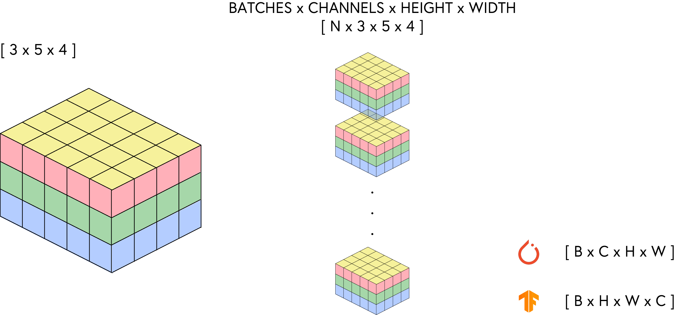
Since images can be seen as 3D tensors, we need to convert them into a format suitable for processing. In PyTorch, images are typically represented as 4D tensors with the shape (batch_size, channels, height, width). For a single image, the shape would be (1, 3, height, width).

To prepare the image data, we will use the torchvision library, which provides convenient functions for loading and transforming images.

3.1 Torchvision transforms

Python uses PIL (Python Imaging Library) to handle images, and while PIL is great for basic image manipulation, it can be slow for large datasets. To speed up the process, we can use torchvision.transforms, which provides a set of common image transformations that can be applied to images in a more efficient way.

Transform	PyTorch Function	Description
Resize	`transforms.Resize(size)`	Resizes the image to the specified size
CenterCrop	`transforms.CenterCrop(size)`	Crops the image at the center to the specified size
RandomCrop	`transforms.RandomCrop(size)`	Crops the image randomly to the specified size
RandomHorizontalFlip	`transforms.RandomHorizontalFlip(p)`	Flips the image horizontally with probability `p`
RandomRotation	`transforms.RandomRotation(degrees)`	Rotates the image randomly within the specified degrees
Normalize	`transforms.Normalize(mean, std)`	Normalizes the image tensor with the specified mean and standard deviation
ColorJitter	`transforms.ColorJitter(brightness, contrast, saturation, hue)`	Randomly changes the brightness, contrast, saturation, and hue of the image
ToTensor	`transforms.ToTensor()`	Converts the image to a PyTorch tensor

These transformations can be combined to create a preprocessing pipeline that prepares the images for training. The transforms.Compose function allows us to chain multiple transformations together.

Notes:

Resizing is important because CNNs require fixed-size inputs.

The ToTensor transformation converts the image to a PyTorch tensor, and it also scales the pixel values to the range [0, 1].

Normalization is a common practice in deep learning to ensure that the input data has a mean of 0 and a standard deviation of 1. This helps the model converge faster during training. ***

Snippet 1: Composing transformations

from torchvision import transforms

ts = transforms.Compose([
    transforms.Resize((224, 224)),  # Resize to 224x224
    transforms.ToTensor(),          # Convert to tensor
    transforms.Normalize(mean=[0.5, 0.5, 0.5], std=[0.5, 0.5, 0.5])  # Normalize
])

# Exercise 3: Implementing Image Transformations 🎯
# In this exercise, you will implement and visualize various image transformations
# commonly used in computer vision tasks

from torchvision import transforms


def apply_transformations(image_path):
    """Apply and visualize various image transformations.

    Args:
        image_path (str or Path): Path to the input image

    Returns:
        dict: Dictionary of transformed images
    """
    # Load the image
    img = Image.open(image_path) if isinstance(
        image_path, (str, Path)) else image_path

    # Define transformations
    # 1. Basic resize to 128x128 
    resize_transform = transforms.Compose([
        # Your code here
        # Your code here
    ])

    # 2. Center crop transformation
    center_crop_transform = transforms.Compose([
        # Your code here: Resize the smaller edge to 150 pixels
        # Your code here: Crop a 100x100 square from the center
        # Your code here
    ])

    # 3. Random crop transformation
    random_crop_transform = transforms.Compose([
        transforms.Resize(150),
        # Your code here: random crop of size 100x100
        # Your code here
    ])

    # 4. Random horizontal flip transformation
    hflip_transform = transforms.Compose([
        transforms.Resize((128, 128)),
        # Your code here: 100% flip probability
        # Your code here
    ])

    # 5. Random rotation transformation
    rotate_transform = transforms.Compose([
        transforms.Resize((128, 128)),
        # Your code here: random rotation
        # Your code here

    ])

    # 6. Color jitter transformation
    color_transform = transforms.Compose([
        transforms.Resize((128, 128)),
        # Your code here: color jitter with brightness, contrast, saturation and hue
        # Your code here
    ])

    # 7. Combined transformations (practical data augmentation)
    combined_transform = transforms.Compose([
        # Your code here: random resized crop of size 128x128
        # Your code here: random horizontal flip 
        # Your code here: random rotation of 15 degrees
        # Your code here: color jitter with brightness and contrast
        transforms.ToTensor()
    ])

    # 8. Normalization transformation
    norm_transform = transforms.Compose([
        transforms.Resize((128, 128)),
        transforms.ToTensor(),
        # Your code here: ImageNet normalization with mean and std [0.485, 0.456, 0.406] and [0.229, 0.224, 0.225]
        # Your code here
    ])

    transforms_list = {
        'Original': transforms.ToTensor(),
        'Resized': resize_transform,
        'Center Crop': center_crop_transform,
        'Random Crop': random_crop_transform,
        'Horizontal Flip': hflip_transform,
        'Random Rotation': rotate_transform,
        'Color Jitter': color_transform,
        'Combined': combined_transform,
        'Normalized': norm_transform
    }

    # Apply transformations
    transforms_dict = {
        'Original': transforms.ToTensor()(img),
        'Resized': resize_transform(img),
        'Center Crop': center_crop_transform(img),
        'Random Crop': random_crop_transform(img),
        'Horizontal Flip': hflip_transform(img),
        'Random Rotation': rotate_transform(img),
        'Color Jitter': color_transform(img),
        'Combined': combined_transform(img),
        'Normalized': norm_transform(img)
    }

    return transforms_dict, transforms_list


# Apply transformations to an image and visualize the results
# Use the ascent image we loaded earlier as a test image
ts_dict, ts_list = apply_transformations(asc_image)
utils.plotting.se04_visualize_transformations(ts_dict)


# ✅ Check your answer
answer = {
    'resize_transform': ts_list['Resized'],
    'center_crop_transform': ts_list['Center Crop'],
    'random_crop_transform': ts_list['Random Crop'],
    'hflip_transform': ts_list['Horizontal Flip'],
    'rotate_transform': ts_list['Random Rotation'],
    'color_transform': ts_list['Color Jitter'],
    'norm_transform': ts_list['Normalized'],
}
checker.check_exercise(3, answer)

3.2 Historical Crack Dataset

In this session, we are going to be working with the Historical-crack18-19 dataset. The dataset contains annotated images for non-invasive surface crack detection in historical buildings. The goal is to train a model that can accurately identify cracks in these images. The current manual visual inspection of built environments is time-consuming, labor-intensive, prone to errors, costly, and lacks scalability. Therefore, the dataset is designed to facilitate the development of deep learning models for automatic crack detection.

The dataset contains:

Attribute	Number of Images
Crack	757
No crack	3,139

As we can see, the dataset is highly imbalanced, with a significant number of images without cracks. This imbalance can affect the performance of the model, as it may learn to predict the majority class (no crack) more often than the minority class (crack). In a first instance, we are going to take a subset of the dataset to balance the classes.

data_path = Path.cwd() / "datasets"
dataset_path = utils.data.download_dataset("historical cracks",
                                   dest_path=data_path,
                                   extract=True,
                                   remove_compressed=True)

img_crack = dataset_path / "crack"
img_no_crack = dataset_path / "non-crack"

# Create a new folder for the balanced dataset
balanced_data_path = dataset_path / "balanced"
balanced_data_path.mkdir(parents=True, exist_ok=True)

# Create train, test, and validation folders
train_folder = balanced_data_path / "train"
train_folder.mkdir(parents=True, exist_ok=True)
test_folder = balanced_data_path / "test"
test_folder.mkdir(parents=True, exist_ok=True)
val_folder = balanced_data_path / "val"
val_folder.mkdir(parents=True, exist_ok=True)

for folder in [train_folder, test_folder, val_folder]:
    (folder / "crack").mkdir(parents=True, exist_ok=True)
    (folder / "no_crack").mkdir(parents=True, exist_ok=True)

crack_images = list(img_crack.glob("*.jpg"))
no_crack_images = random.sample(list(img_no_crack.glob("*.jpg")), len(crack_images))

# Shuffle the images
random.shuffle(crack_images)
random.shuffle(no_crack_images)

# Split the images into train, test, and validation sets
train_ix = int(0.8 * len(crack_images))
val_ix = int(0.9 * len(crack_images))
test_ix = len(crack_images)

train_crack_images = crack_images[:train_ix]
val_crack_images = crack_images[train_ix:val_ix]
test_crack_images = crack_images[val_ix:test_ix]

train_no_crack_images = no_crack_images[:train_ix]
val_no_crack_images = no_crack_images[train_ix:val_ix]
test_no_crack_images = no_crack_images[val_ix:test_ix]

# Copy the images to the new folders
for img in train_crack_images:
    shutil.copy(img, train_folder / "crack")
for img in train_no_crack_images:
    shutil.copy(img, train_folder / "no_crack")
for img in val_crack_images:
    shutil.copy(img, val_folder / "crack")
for img in val_no_crack_images:
    shutil.copy(img, val_folder / "no_crack")
for img in test_crack_images:
    shutil.copy(img, test_folder / "crack")
for img in test_no_crack_images:
    shutil.copy(img, test_folder / "no_crack")

# Randomly select 5 images
random_images = random.sample(crack_images, 5)

# Display the images
fig, axes = plt.subplots(1, 5, figsize=(15, 5))
for ax, img_path in zip(axes, random_images):
    img = Image.open(img_path)
    ax.imshow(img)
    ax.axis('off')
    ax.set_title(img_path.stem)
plt.tight_layout()

print (f"Images size: {img.size}")

3.3 PyTorch ImageFolder

While we can load images using PIL, PyTorch provides a more efficient way to handle large datasets through the torchvision.datasets module. This module contains the ImageFolder class, which allows us to load images from a directory structure where each subdirectory represents a class. The ImageFolder class automatically assigns labels based on the subdirectory names.

The ImageFolder class requires a root directory containing subdirectories for each class. The directory structure should look like this:

dataset/
    ├── class-1/
    │   ├── image1.jpg
    │   ├── image2.jpg
    │   └── ...
    └── class-2/
        ├── image1.jpg
        ├── image2.jpg
        └── ...

The function automatically assigns labels to the images based on the subdirectory names. Moreover, it can also apply transformations to the images using the transform parameter.

The key parameters of the ImageFolder class are:

Parameter	Description
root	The root directory containing the dataset
transform	A function/transform to apply to the images
target_transform	A function/transform to apply to the target (label)
loader	A function to load the images (default is `PIL.Image.open`)
is_valid_file	A function to check if a file is valid (default is `None`)

Snippet 2: Using ImageFolder

from torchvision.datasets import ImageFolder

dataset = ImageFolder(root='path/to/dataset', transform=ts)
# Accessing the first image and its label
image, label = dataset[0]
print(f"Image shape: {image.shape}, Label: {label}")

# Exercise 4: Data Augmentation and Loading with PyTorch 🎯
# Implement:
# 1. Data augmentation techniques
# 2. Data loading with ImageFolder

from torch.utils.data import random_split, DataLoader
from torchvision.datasets import ImageFolder

ts_train = transforms.Compose([
    # Your code here: Add transforms for training data
    # Resize to 64x64, add random horizontal flip
    # Add random rotation, add color jitter
    # Convert to tensor
    # Your code here
])

ts_test_val = transforms.Compose([
    # Your code here: Add transforms for test/val data
    # We only need to resize and convert to tensor for test/val
    # Your code here
])

# Create datasets using ImageFolder
train_data = # Your code here
test_data = # Your code here
val_data = # Your code here


# ✅ Check your answer
answer = {
    'train_transforms': ts_train,
    'test_val_transforms': ts_test_val,
    'train_data': train_data,
    'test_data': test_data,
    'val_data': val_data
}
checker.check_exercise(4, answer)

3.4 PyTorch DataLoaders

As we discussed in the previous session, when training a model we need to load the data in batches. PyTorch provides the DataLoader class to handle this efficiently. The DataLoader class takes a dataset and provides an iterable over the dataset, allowing us to load data in batches.

The model expects our image data to be formatted as a 4D tensor with the shape (batch_size, channels, height, width).

The DataLoader class provides several key parameters to customize the data loading process:

Parameter	Description
dataset	The dataset to load data from (e.g., `ImageFolder`)
batch_size	The number of samples per batch
shuffle	Whether to shuffle the data at every epoch
num_workers	The number of subprocesses to use for data loading
pin_memory	Whether to pin memory for faster data transfer to GPU
drop_last	Whether to drop the last incomplete batch

Snippet 3: Creating a DataLoader

from torch.utils.data import DataLoader

# Create a DataLoader for the dataset
train_loader = DataLoader(dataset, batch_size=32, shuffle=True, num_workers=4, pin_memory=True)
# Iterate through the DataLoader
for images, labels in train_loader:
    print(f"Batch shape: {images.shape}, Labels: {labels}")
    break  # Just to show the first batch

# Exercise 5: DataLoader 🎯
# Create DataLoaders for train, test, and validation data

# Your code here: create train_dl with batch_size=32 and shuffle=True
train_dl = # Your code here
# Your code here: create test_dl with batch_size=32 and shuffle=False
test_dl = # Your code here
# Your code here: create val_dl with batch_size=32 and shuffle=False
val_dl = # Your code here

# ✅ Check your answer
answer = {
    'train_dataloader': train_dl,
    'test_dataloader': test_dl,
    'val_dataloader': val_dl,
    'batch_size': train_dl.batch_size
}
checker.check_exercise(5, answer)

4. Implementing CNNs

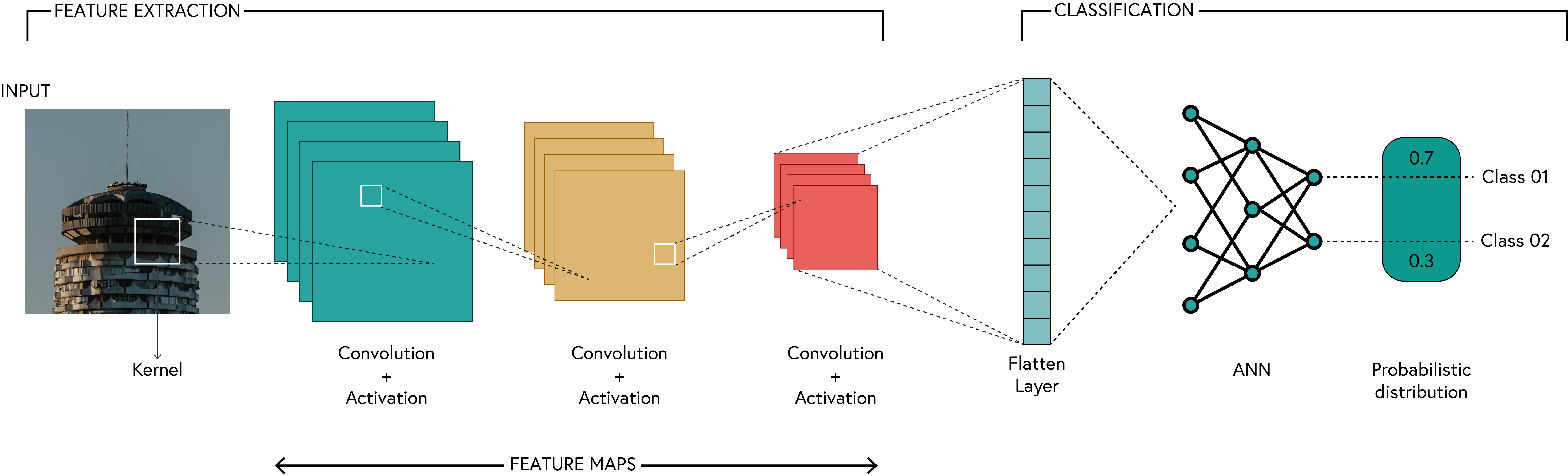
The architecture of a CNN is not that different from a standard neural network. The main difference is that CNNs use convolutional layers instead of fully connected layers. This means that after each convolutional layer, we typically apply a non-linear activation function (like ReLU).

The output of the CNN is then passed through one or more fully connected layers to produce the final output. Thus, we need to keep track of the output size after each layer to ensure that the dimensions match up correctly.

A diagram of a conventional CNN architecture is shown below.

We are going to implement a simple CNN architecture for the crack detection task. The architecture consists of the following layers:

Type	Layer	Input Size	Output Size	Activation Function
Convolution	`Conv2d`	`(3, 64, 64)`	`(16, 64, 64)`	ReLU
Fully Connected	`Linear`	`(16 * 64 * 64)`	`16`	ReLU
Fully Connected	`Linear`	`16`	`2`	None

# Exercise 6: Implementing a Simple CNN Model 🎯
class simpleCNN(torch.nn.Module):
    def __init__(self, n_classes):
        super(simpleCNN, self).__init__()
        # Your code here: create a convolutional layer with 3 input channels, 16 output channels
        # kernel_size=3, stride=1, padding=1
        self.conv1 = # Your code here
        # Your code here: create a fully connected layer (Linear) with input 16*64*64 and output 16
        self.fc1 = # Your code here
        # Your code here: create a fully connected layer (Linear) with input 16 and output n_classes
        self.fc2 = # Your code here

    def forward(self, x):
        # Your code here: Apply ReLU activation to conv1 output
        x = # Your code here
        # Your code here: Flatten the tensor
        x = # Your code here
        # Your code here: Apply ReLU activation to fc1 output
        x = # Your code here
        # Your code here: Feed through fc2
        x = # Your code here
        return x

model_v1 = simpleCNN(len(train_data.classes))
criterion = torch.nn.CrossEntropyLoss()
optimiser = torch.optim.Adam(model_v1.parameters(), lr=3e-3)
num_epochs = 10

# ✅ Check your answer
answer = {
    'model_architecture': model_v1,
    'conv_layer': model_v1.conv1,
    'linear_layers': {'count': 2, 'output_features': model_v1.fc2.out_features},
    'activation': {'function': 'ReLU', 'count': 2},
}
checker.check_exercise(6, answer)

model_v1 = utils.ml.train_model(model_v1,
                                criterion,
                                optimiser,
                                train_loader=train_dl,
                                val_loader=val_dl,
                                num_epochs=num_epochs,
                                plot_loss=True)

4.1 Getting predictions

The output of the last layer gives us the predicted class probabilities for the two classes: crack and no crack. Therefore, in order for us to get the predicted class, we need to apply a softmax function to the output of the last layer. However, PyTorch CrossEntropyLoss combines the softmax and the negative log-likelihood loss in a single function, so we don’t need to apply softmax explicitly. The CrossEntropyLoss function expects the raw logits (the output of the last layer) as input, and it will apply softmax internally.

To predict the class, we can use the torch.argmax function to get the index of the maximum value in the output tensor. This index corresponds to the predicted class.

Snippet 4: Obtaining the predicted class

model_v1.eval()

with torch.no_grad():
    for images, labels in test_dl:
        outputs = model_v1(images.to(device))
        print(outputs[:-1])
        _, predicted = torch.max(outputs, dim=1)
        print(predicted)
        break

# Exercise 7: Evaluating the Model 🎯
# Compute accuracy and classification report

# Your code here: Use the utils.ml.compute_accuracy function to compute accuracy on the test set
acc = # Your code here
print(f"Test accuracy: {acc*100:.2f}%")

# Your code here: Use the utils.ml.compute_classification_report function to compute the classification report
cls_report = # Your code here
print('-' * 60)
print(f"Classification Report:\n{cls_report}")

# ✅ Check your answer
answer = {
    'test_accuracy': acc,
    'classification_report': cls_report
}
checker.check_exercise(7, answer)

# Visualize the model predictions
utils.plotting.show_model_predictions(model_v1, test_dl, class_names=train_data.classes)

4.2 Recreating CNN architectures

There are many different CNN architectures that have been proposed in the literature, each with its own strengths and weaknesses. Some of the most popular architectures include:

Architecture	Description	Key Features
LeNet	One of the first CNN architectures, designed for handwritten digit recognition	5 layers, small kernel sizes
AlexNet	A deeper architecture that won the ImageNet competition in 2012	8 layers, ReLU activation, dropout, data augmentation
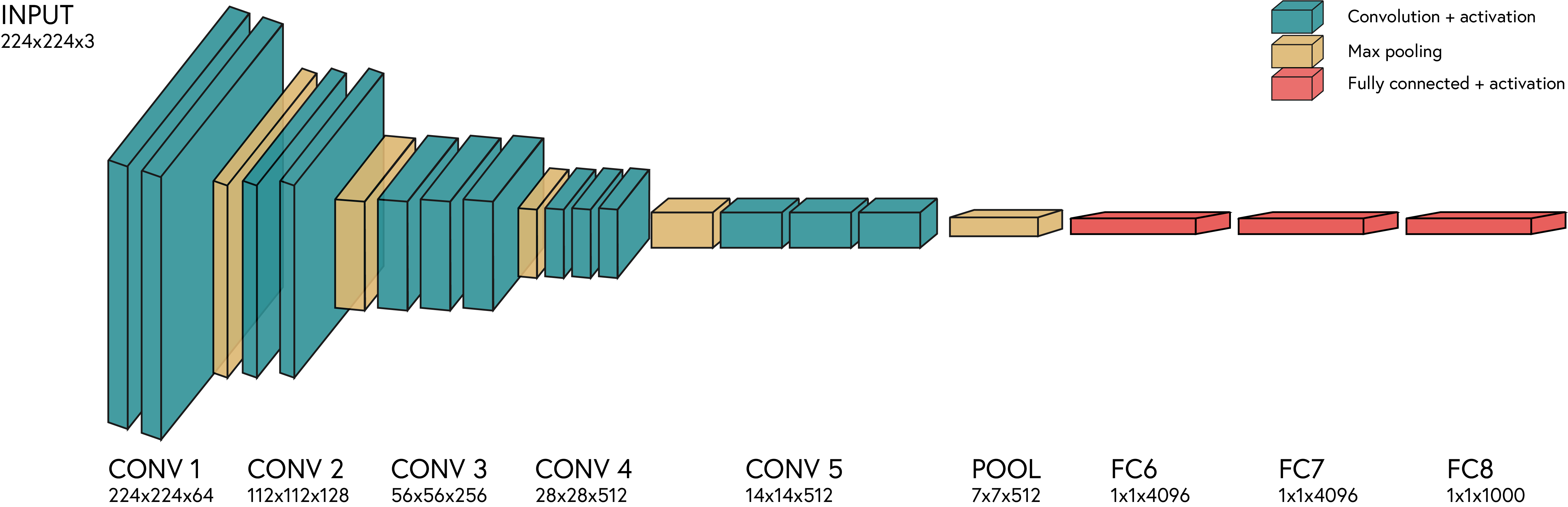
VGG	A very deep architecture with small kernel sizes	16-19 layers, uniform architecture, small kernels
ResNet	Introduced residual connections to allow for very deep networks	50-152 layers, skip connections, batch normalization
Inception	Introduced the inception module for multi-scale feature extraction	22-164 layers, parallel convolutions, pooling layers
DenseNet	Introduced dense connections between layers	121-201 layers, dense connections, feature reuse

These architectures have been shown to perform well on a variety of tasks, and they can be used as a starting point for building custom CNNs. Furthermore, many of these architectures are often visualised as a series of blocks, where each block consists of a convolutional layer followed by an activation function and a pooling layer. We are going to implement a version of the original VGG architecture, which looks like this:

4.3 Pooling

Definition: Pooling is a downsampling operation used in CNNs to reduce the spatial dimensions of feature maps while retaining important information.

Pooling helps to reduce the number of parameters and computations in the network, making it more efficient and less prone to overfitting. There are several types of pooling operations, but the most common ones are:

Pooling Type	PyTorch Function	Description
Max Pooling	`torch.nn.MaxPool2d(kernel_size, stride)`	Takes the maximum value in each region defined by the kernel size
Average Pooling	`torch.nn.AvgPool2d(kernel_size, stride)`	Takes the average value in each region defined by the kernel size
Global Average Pooling	`torch.nn.AdaptiveAvgPool2d(output_size)`	Reduces each feature map to a single value by averaging over the entire map
Global Max Pooling	`torch.nn.AdaptiveMaxPool2d(output_size)`	Reduces each feature map to a single value by taking the maximum over the entire map

The pooling operation can be visualised like this:

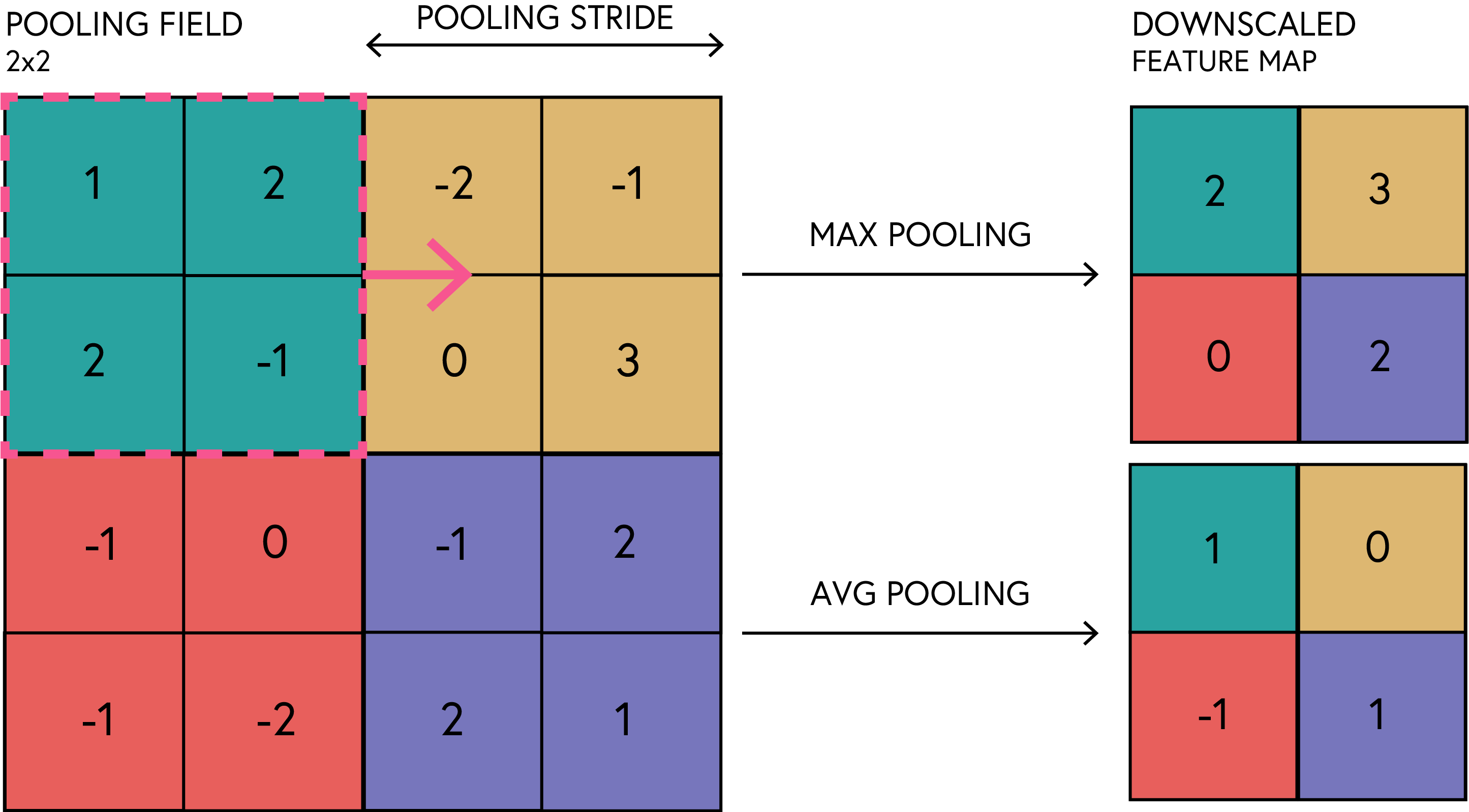
Most commonly, we use max pooling, as it helps to retain the most important features while discarding less relevant information. The pooling operation is typically applied after a convolutional layer and an activation function.

4.4 Regularisation

As briefly mentioned in the previous session, regularisation is a technique used to prevent overfitting in machine learning models. Overfitting occurs when a model learns the training data too well, including noise and outliers, leading to poor generalisation on unseen data. In CNNs, regularisation techniques are crucial due to the large number of parameters and the complexity of the models. Some common regularisation techniques used in CNNs include:

Regularisation Technique	Pytorch Function	Description
Dropout	`torch.nn.Dropout(p)`	Randomly sets a fraction of input units to 0 at each update during training time, which helps prevent overfitting
L2 Regularisation	`torch.nn.functional.mse_loss()`	Adds a penalty on the size of the weights to the loss function. This is also known as weight decay
Batch Normalisation	`torch.nn.BatchNorm2d(num_features)`	Normalises the output of a previous activation layer by subtracting the batch mean and dividing by the batch standard deviation. This helps to stabilise the learning process and can lead to faster convergence
Data Augmentation	`torchvision.transforms`	Increases the diversity of the training set by applying random transformations to the input data, such as rotation, translation, and scaling. This helps to improve the generalisation of the model
Early Stopping	`torch.nn.utils`	Stops training when the validation loss stops improving, preventing overfitting
Weight Decay	`torch.optim.AdamW`	Adds a penalty on the size of the weights to the loss function, similar to L2 regularisation. This is also known as weight decay

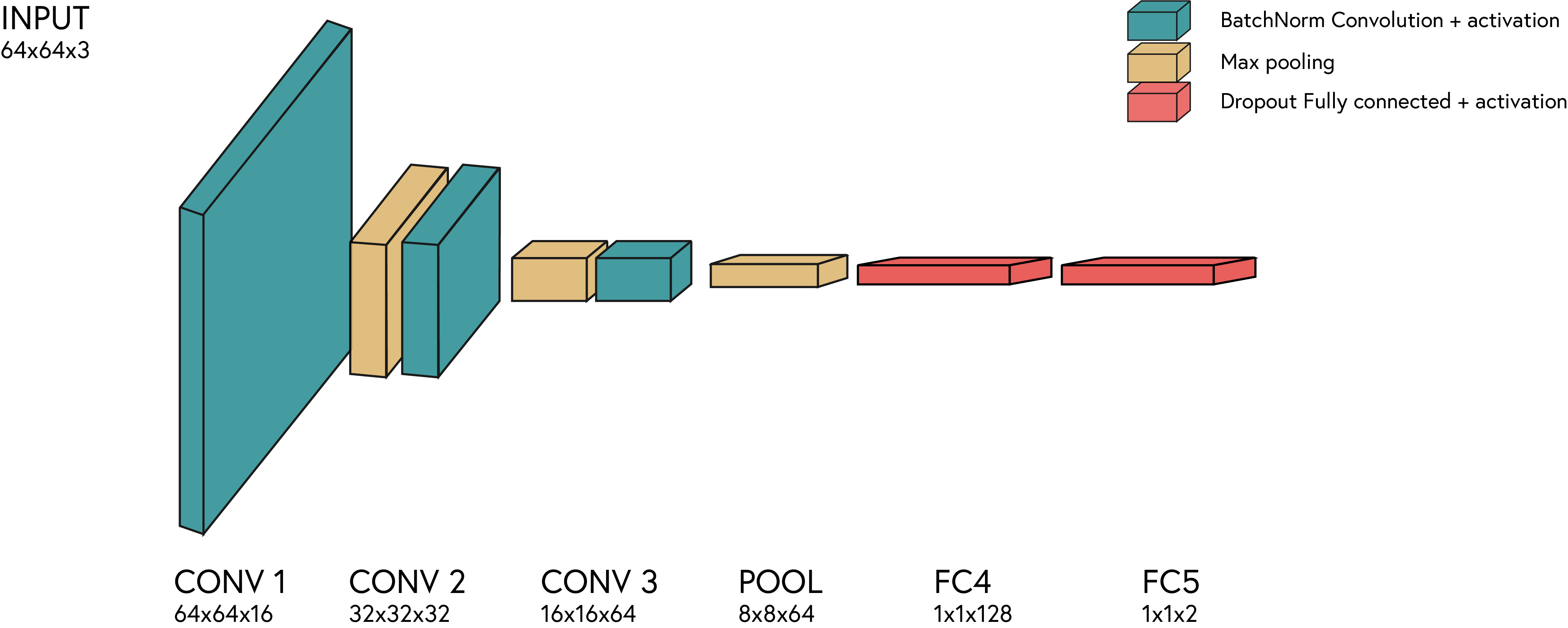
For our tiny VGG architecture, we are going to use dropout and batch normalisation. The dropout layer is applied after the activation function of the fully connected layers, while the batch normalisation layer is applied after the convolutional layers.

Our tiny VGG architecture will look like this:

# Exercise 8: Implementing a More Complex CNN Model 🎯
class tinyVGG(torch.nn.Module):
    def __init__(self, n_classes):
        super().__init__()
        # Create convolutional layers
        # Your code here: conv1 with 3 input channels, 16 output channels
        self.conv1 = # Your code here
        # Your code here: conv2 with 16 input channels, 32 output channels
        self.conv2 = # Your code here
        # Your code here: conv3 with 32 input channels, 64 output channels
        self.conv3 = # Your code here
        
        # Add pooling layers
        # Your code here: Create max pooling layer with kernel_size=2, stride=2
        self.pool = # Your code here
        
        # Your code here: Create flatten layer
        self.flat = # Your code here
        # Adjust input size for fully connected layer due to pooling
        # Your code here: Create fc1 with input 64*8*8 and output 128
        self.fc1 = # Your code here
        # Your code here: Create fc2 with input 128 and output n_classes
        self.fc2 = # Your code here
        
        # dropout for regularization
        # Your code here: Create dropout1 with p=0.05
        self.dropout1 = # Your code here
        # Your code here: Create dropout2 with p=0.1
        self.dropout2 = # Your code here
        
        # batch normalization for more stable training
        # Your code here: Create batch_norm1 for 16 features
        self.batch_norm1 = # Your code here
        # Your code here: Create batch_norm2 for 32 features
        self.batch_norm2 = # Your code here
        # Your code here: Create batch_norm3 for 64 features
        self.batch_norm3 = # Your code here

    def forward(self, x):
        # Your code here: Apply conv1, batch_norm1, ReLU, and pooling
        x = # Your code here
        x = # Your code here
        # Your code here: Apply conv2, batch_norm2, ReLU, and pooling
        x = # Your code here
        x = # Your code here
        # Your code here: Apply conv3, batch_norm3, ReLU, and pooling
        x = # Your code here
        x = # Your code here
        # Your code here: Flatten the tensor
        x = # Your code here
        # Your code here: Apply fc1, ReLU, and dropout2
        x = # Your code here
        # Your code here: Apply fc2
        x = # Your code here
        return x


# ✅ Check your answer
model_v2 = tinyVGG(len(train_data.classes))
answer = {
    'model_architecture': model_v2,
    'conv_layers': model_v2,
    'pooling_layers': model_v2.pool,
    'batch_norm_layers': [model_v2.batch_norm1, model_v2.batch_norm2, model_v2.batch_norm3],
    'dropout_layers': [model_v2.dropout1, model_v2.dropout2],
    'flatten_operation': model_v2.flat
}
checker.check_exercise(8, answer)

model_v2 = tinyVGG(len(train_data.classes))
criterion_reg = torch.nn.CrossEntropyLoss()
optimiser_reg = torch.optim.Adam(model_v2.parameters(),
                                 lr=1e-3,
                                 betas=(0.9, 0.999),
                                #  weight_decay=1e-5,  # L2 regularization (weight decay)
                                 ) 
num_epochs_reg = 45
scheduler = torch.optim.lr_scheduler.ReduceLROnPlateau(
    optimiser_reg,
    mode='min',
    factor=0.1,
    patience=2,
)

model_v2 = utils.ml.train_model(model_v2,
                  criterion_reg,
                  optimiser_reg,
                  train_loader=train_dl,
                  val_loader=val_dl,
                  num_epochs=num_epochs_reg,
                  early_stopping=True,
                  patience=5,
                  tolerance=1e-2,
                  save_path= Path.cwd() / "my_models" / "se04_model_v2.pt",
                  plot_loss=True)

# Load the best model
model_v2.load_state_dict(torch.load(Path.cwd() / "my_models" / "se04_model_v2.pt"))

# Exercise 9: Evaluating the tiny VGG🎯
# Your code here: Use the utils.ml.compute_accuracy function to compute accuracy on the test set
acc = # Your code here
print(f"Test accuracy: {acc*100:.2f}%")

# Your code here: Use the utils.ml.compute_classification_report function to compute the classification report
cls_report = # Your code here
print('-' * 60)
print(f"Classification Report:\n{cls_report}")

# ✅ Check your answer
answer = {
    'test_accuracy': acc,
    'classification_report': cls_report
}
checker.check_exercise(9, answer)

utils.plotting.show_model_predictions(model_v2, test_dl, class_names=train_data.classes, num_images=12)

Filter	Kernel	Description
Edge Detection	\(\begin{bmatrix} 1 & 0 & -1 \\ 1 & 0 & -1 \\ 1 & 0 & -1 \end{bmatrix}\)	Detects vertical edges
Sharpening	\(\begin{bmatrix} 0 & -1 & 0 \\ -1 & 5 & -1 \\ 0 & -1 & 0 \end{bmatrix}\)	Enhances edges and details
Embossing	\(\begin{bmatrix} -2 & -1 & 0 \\ -1 & 1 & 1 \\ 0 & 1 & 2 \end{bmatrix}\)	Creates a 3D effect