
# Download utils from GitHub
!wget -q --show-progress https://raw.githubusercontent.com/CLDiego/uom_fse_dl_workshop/main/colab_utils.txt -O colab_utils.txt
!wget -q --show-progress -x -nH --cut-dirs=3 -i colab_utils.txt
from pathlib import Path
import sys
repo_path = Path.cwd()
if str(repo_path) not in sys.path:
sys.path.append(str(repo_path))
import utils
import numpy as np
import inspect
from torchvision import transforms
from PIL import Image
import random
import torch
# Set random seeds for reproducibility
torch.manual_seed(101)
torch.cuda.manual_seed(101)
random.seed(101)
torch.backends.cudnn.deterministic = True
torch.backends.cudnn.benchmark = False
print("GPU available:", torch.cuda.is_available())
if torch.cuda.is_available():
print("GPU device:", torch.cuda.get_device_name(0))
else:
print("No GPU available. Please ensure you've enabled GPU in Runtime > Change runtime type")
checker = utils.core.ExerciseChecker("SE05")
quizzer = utils.core.QuizManager("SE05")1. Introduction to Transfer Learning
Definition: Transfer learning is a machine learning technique where a model developed for one task is reused as a starting point for a model on a second task. It’s particularly effective for deep learning models, as it allows us to leverage pre-trained models’ knowledge rather than starting from scratch.
In previous sessions, we learned how to build and train neural networks from scratch. However, training large deep learning models requires:
- Massive datasets (often millions of examples)
- Extensive computational resources (often multiple GPUs)
- Long training times (days to weeks)
Transfer learning addresses these challenges by letting us capitalise on existing models that have already been trained on large datasets.
1.1 Transfer Learning Analogy
Transfer learning is inspired by human learning. Consider how we learn:
| Human Learning | Machine Learning Parallel |
|---|---|
| A child learns to recognize basic shapes before identifying letters | A model learns edge detection before specific object recognition |
| A musician who knows piano can learn guitar faster than a novice | A model trained on one image dataset can adapt quickly to a similar task |
| Language skills transfer across related languages (e.g., Spanish to Italian) | NLP models pre-trained on one language can be fine-tuned for another |
| Medical students learn general anatomy before specializing | Medical imaging models trained on general X-rays can be fine-tuned for specific conditions |
| Engineers apply fundamental principles across different projects | Engineering models transfer physical principles across different applications |
This mirrors how neural networks learn hierarchical features. Early layers learn general patterns that are often applicable across domains, while later layers learn task-specific features.
1.2 When to Use Transfer Learning
Transfer learning is particularly useful in the following scenarios:
| Scenario | Example | Benefit |
|---|---|---|
| Limited training data | Medical imaging with few samples | Pre-trained features compensate for data scarcity |
| Similar domains | From natural images to satellite imagery | Underlying features (edges, textures) transfer well |
| Time constraints | Rapid prototyping needs | Accelerates model development cycle |
| Hardware limitations | Training with limited GPU access | Reduces computational requirements |
| Preventing overfitting | Small dataset applications | Regularization effect from pre-trained weights |
Key Insight: The effectiveness of transfer learning depends on the similarity between the source and target domains. The more similar they are, the more beneficial transfer learning becomes.
# Quiz on Transfer Learning Concepts
print("\n🧠 Quiz 1: Transfer Learning Applications")
quizzer.run_quiz(1)
2. Case Study: Image Segmentation for Medical Imaging
For this session, we are going to be using the ISIC 2016 Skin Lesion Segmentation Challenge dataset. This dataset contains dermoscopic images of skin lesions, along with their corresponding segmentation masks. The goal is to train a model to accurately segment the lesions from the background.
data_path = Path(Path.cwd(), 'datasets')
dataset_path = utils.data.download_dataset('skin lesions',
                                           dest_path=data_path,
                                           extract=True,
                                           remove_compressed=False)

mask_path = utils.data.download_dataset('skin lesions masks',
                                   dest_path=data_path,
                                   extract=True,
                                   remove_compressed=False)

test_path = utils.data.download_dataset('skin lesions test',
                                   dest_path=data_path,
                                   extract=True,
                                   remove_compressed=False)

test_mask_path = utils.data.download_dataset('skin lesions test masks',
                                   dest_path=data_path,
                                   extract=True,
                                   remove_compressed=False)
2.1 Challenges in Medical Image Segmentation
Medical image segmentation presents unique challenges compared to natural image segmentation:
| Challenge | Description | Impact |
|---|---|---|
| Limited Data | Medical datasets are typically smaller | Transfer learning becomes crucial |
| Class Imbalance | Regions of interest often occupy a small portion of the image | Requires specialized loss functions |
| Ambiguous Boundaries | Boundaries between tissues can be gradual or unclear | Makes precise segmentation difficult |
| Inter-observer Variability | Different experts may segment the same image differently | Ground truth is not always definitive |
| High Stakes | Errors can have serious consequences in medical applications | Demands higher accuracy and reliability |
3. Preparing the Dataset
Segmentation tasks require both the input images and their corresponding masks. The masks are binary images where the pixels belonging to the object of interest (e.g., a tumor) are marked as 1 (or white), while the background is marked as 0 (or black). Thus, we need to load both the images and their masks for training.
3.1 Custom Dataset Creation
In order for us to efficiently load the images and masks, we are going to create a custom dataset class. This class will inherit from the torch.utils.data.Dataset class and will handle loading the images and masks from the specified directories.
The PyTorch Dataset class is an abstract class representing a dataset. Custom datasets should inherit from this class and override the following methods:
| Method | Purpose | Implementation Requirements |
|---|---|---|
__init__ |
Initialize the dataset | Define directories, transformations, and data loading parameters |
__len__ |
Return dataset size | Return the total number of samples |
__getitem__ |
Access a specific sample | Load and transform a sample with a given index |
For image segmentation, our dataset needs to handle both input images and their corresponding segmentation masks:
Snippet 1: Create a custom dataset class for loading
from torch.utils.data import Dataset

class CustomDataset(Dataset):
    def __init__(self, **kwargs):
        """
        Initializes the dataset, loading the images and masks from the specified directories.
        """

    def __len__(self):
        """
        Returns the number of images in the dataset.
        """

    def __getitem__(self, idx):
        """
        Defines how to get a single item (image and mask) from the dataset.
# Exercise 1: Creating a Custom Dataset 🎯
# Implement:
# 1. Create a custom dataset class for the ISIC dataset.
# 2. Implement the __len__ and __getitem__ methods.
# 3. Use the PIL library to read images and masks.
# 4. Apply transformations to images and masks if provided.

from torch.utils.data import Dataset, DataLoader

class ISICDataset(Dataset):
    def __init__(self, image_dir: Path | str, mask_dir: Path | str, img_transform=None, mask_transform=None):
        self.image_dir = Path(image_dir)
        self.mask_dir = Path(mask_dir)
        self.img_transform = img_transform
        self.mask_transform = mask_transform
        # Your code here: Get list of image files from the image directory (use sorted and glob)
        self.images = # Your code here
        # Your code here: Get list of mask files from the mask directory
        self.masks = # Your code here

    def __len__(self):
        # Your code here: Return the number of images in the dataset
        return # Your code here

    def __getitem__(self, idx):
        # Your code here: Get the image and mask filenames at the specified index
        img_name = # Your code here
        img_path = # Your code here
        mask_name = # Your code here: Format should be "img_name_stem + _Segmentation.png"
        mask_path = # Your code here

        # Your code here: Open the image and convert to RGB
        image = # Your code here
        # Your code here: Open the mask and convert to grayscale (single channel)
        mask = # Your code here

        # Apply transformations if provided
        if self.img_transform:
            # Your code here: Apply image transformation
            image = # Your code here
        if self.mask_transform:
            # Your code here: Apply mask transformation
            mask = # Your code here

        return image, mask

resize_transform = transforms.Compose([
    transforms.Resize((64, 64)),
    transforms.ToTensor(),
])

ds = ISICDataset(
    image_dir=dataset_path,
    mask_dir=mask_path,
    img_transform=resize_transform,
    mask_transform=resize_transform
)
# ✅ Check Exercise 1: Custom Dataset Implementation
answer = {
'has_getitem': hasattr(ISICDataset, '__getitem__'),
'has_len': hasattr(ISICDataset, '__len__'),
'dataset_instance': ds,
'img_transform_used': hasattr(ds, 'img_transform') and ds.img_transform is not None,
'mask_transform_used': hasattr(ds, 'mask_transform') and ds.mask_transform is not None
}
checker.check_exercise(1, answer)3.2 Compute the Mean and Standard Deviation of the Dataset
Computing dataset statistics is a critical step in preparing data for deep learning models. We need to normalize our images to help the model converge faster and perform better. By normalizing with the dataset’s mean and standard deviation, we ensure that the input values have similar scales and distributions.
The normalisation process follows this formula for each channel:
\[x_{normalized} = \frac{x - \mu}{\sigma}\]Where:
- $x$ is the original pixel value
- $\mu$ is the mean of all pixels in the channel across the dataset
- $\sigma$ is the standard deviation of all pixels in the channel across the dataset
First, we need to load the dataset and then compute the mean and standard deviation across all images.
# Exercise 2: Calculating Mean and Std of Images 🎯
# Implement:
# 1. Create a DataLoader for the dataset.
# 2. Iterate through the DataLoader to calculate the mean and standard deviation of the images.

from tqdm import tqdm

# Your code here: Create a DataLoader with batch size 16 and shuffle=False
dl = # Your code here
device = torch.device("cuda" if torch.cuda.is_available() else "cpu")

n_channels = 3
n_pixels = 0
# Your code here: Initialize tensors to store channel sums and squared sums
channel_sum = # Your code here
channel_squared_sum = # Your code here

for images, _ in tqdm(dl, desc="Calculating mean and std"):
    # Your code here: Reshape images to (batch_size, channels, height*width)
    images = # Your code here
    # Your code here: Update the number of pixels
    n_pixels += # Your code here

    # Your code here: Update sums (sum over batch and pixels dimensions)
    channel_sum += # Your code here
    # Your code here: Update squared sums
    channel_squared_sum += # Your code here

# Calculate mean and std
# Your code here: Calculate mean as sum divided by number of pixels
mean = # Your code here
# Your code here: Calculate std using formula: sqrt((sum_of_squares / count) - mean^2)
std = # Your code here

print("Mean:", mean)
print("Std:", std)
# ✅ Check Exercise 2: Mean and Standard Deviation Calculation
answer = {
'dataloader': dl,
'mean_shape': mean.shape,
'std_shape': std.shape,
'mean_range': torch.all((mean >= 0) & (mean <= 1)).item(),
'std_range': torch.all((std > 0) & (std < 1)).item()
}
checker.check_exercise(2, answer)3.3 Data Augmentation
We are going to use the albumentations library for data augmentation. This library outperforms the torchvision library in terms of speed and flexibility. It provides the same transformations as torchvision and it is also compatible with PyTorch.
3.3.1 Choosing Appropriate Augmentations for Medical Images
| Augmentation Type | Purpose | Medical Imaging Considerations |
|---|---|---|
| Geometric Transforms | Rotate, flip, resize | Should preserve diagnostic features |
| Color Adjustments | Brightness, contrast, saturation | Use carefully to maintain diagnostic appearance |
| Noise Addition | Add random noise | Models will be more robust to image noise |
| Elastic Deformations | Simulate tissue deformation | Especially useful for soft tissue imaging |
| Cropping | Focus on different regions | Ensures focus on different areas of lesion |
3.3.2 Sync vs. Async Augmentation
For segmentation tasks, we need to ensure that the same transformations are applied to both the image and its corresponding mask. This is called synchronized (sync) augmentation, as opposed to asynchronous (async) augmentation where different transformations are applied to inputs and targets.
| Type | Description | Use Case |
|---|---|---|
| Sync Augmentation | Apply identical spatial transforms to image and mask | Required for segmentation tasks |
| Async Augmentation | Apply different transforms | Typically used for classification only |
import albumentations as A
from albumentations.pytorch import ToTensorV2

transform = A.Compose([
    A.HorizontalFlip(p=0.5),
    A.VerticalFlip(p=0.5),
    A.RandomRotate90(p=0.5),
    A.RandomBrightnessContrast(p=0.2),
    A.Normalize(mean=mean, std=std, p=1.0),
    ToTensorV2()
])
# Exercise 3: Data Augmentation with Albumentations 🎯
# Implement:
# 1. Use the Albumentations library to apply data augmentation techniques.
# 2. Create a transformation pipeline for training and validation datasets.
# 3. The training pipeline should include:
#    - Resize to 64x64
#    - Random horizontal and vertical flips
#    - Random rotation (limit 10 degrees)
#    - Random brightness, contrast, saturation, and hue adjustments
#    - Normalization using the calculated mean and std
# 4. The validation pipeline should include:
#    - Resize to 64x64
#    - Normalization using the calculated mean and std
# 5. All transformations should convert images to PyTorch tensors.

import albumentations as A
from albumentations.pytorch import ToTensorV2

# Your code here: Create training transforms pipeline with all required augmentations
train_img_ts = A.Compose([
    # Your code here: Resize to 64x64
    # Your code here: HorizontalFlip with 50% probability
    # Your code here: VerticalFlip with 50% probability
    # Your code here: Random rotation with limit=10 and 50% probability
    # Your code here: Color jitter (brightness, contrast, saturation, hue)
    # Your code here: Normalize with mean and std
    # Your code here: Convert to PyTorch tensor
])

# Your code here: Create validation transforms pipeline (simpler, no augmentations)
valid_img_ts = A.Compose([
    # Your code here: Resize to 64x64
    # Your code here: Normalize with mean and std
    # Your code here: Convert to PyTorch tensor
])
# ✅ Check Exercise 3: Data Augmentation with Albumentations
answer = {
'train_transforms': train_img_ts,
'valid_transforms': valid_img_ts,
'has_resize': any(isinstance(t, A.Resize) for t in train_img_ts.transforms),
'has_horizontal_flip': any(isinstance(t, A.HorizontalFlip) for t in train_img_ts.transforms),
'has_vertical_flip': any(isinstance(t, A.VerticalFlip) for t in train_img_ts.transforms),
'has_rotation': any(isinstance(t, A.Rotate) for t in train_img_ts.transforms),
'has_color_jitter': any(isinstance(t, A.ColorJitter) for t in train_img_ts.transforms),
'has_normalize': any(isinstance(t, A.Normalize) for t in train_img_ts.transforms),
'has_to_tensor': any(isinstance(t, ToTensorV2) for t in train_img_ts.transforms)
}
checker.check_exercise(3, answer)3.3.4 Modifying the Dataset Class to use Albumentations
Since normal PyTorch transforms do not support the synchronized augmentation, we need to modify our dataset class to use albumentations. We will also add the normalization step in the __getitem__ method.
We are going to create a new class called that inherits from our ISICDataset class. This will allow us to override the __getitem__ method and apply the albumentations transformations.
# Exercise 4: Implementing the Albumentations Dataset Class 🎯
# Implement:
# 1. Inherit from the ISICDataset class.
# 2. Override the __getitem__ method to apply Albumentations transformations.
# 3. Ensure the mask is binary (0 or 1)

class ISICDatasetAlbumentations(ISICDataset):
    def __init__(self, image_dir: Path | str, mask_dir: Path | str, transform=None):
        # Your code here: Initialize the parent class
        super().__init__(image_dir, mask_dir, transform, None)

    def __getitem__(self, idx):
        # Your code here: Get the image path
        img_name = # Your code here
        img_path = # Your code here
        # Your code here: Get the mask path
        mask_name = # Your code here
        mask_path = # Your code here

        # Your code here: Open the image and convert to RGB
        image = # Your code here
        # Your code here: Convert to numpy array for albumentations
        image = # Your code here
        # Your code here: Open the mask and convert to grayscale
        mask = # Your code here
        # Your code here: Convert to numpy array
        mask = # Your code here

        # Your code here: Normalize mask to 0-1 range if needed
        if mask.max() > 1:
            # Your code here

        # Your code here: Apply transformations if provided
        if self.img_transform:
            # Your code here: Apply albumentations transform to both image and mask
            aug = # Your code here
            image = # Your code here
            mask = # Your code here

            # Your code here: Ensure mask is binary (0 or 1)
            if isinstance(mask, torch.Tensor):
                # Your code here

        return image, mask
# ✅ Check Exercise 4: Albumentations Dataset Implementation
answer = {
'inherits_from_isic': issubclass(ISICDatasetAlbumentations, ISICDataset),
'has_getitem_override': ISICDatasetAlbumentations.__getitem__ != ISICDataset.__getitem__,
'uses_numpy': 'np.array' in str(inspect.getsource(ISICDatasetAlbumentations.__getitem__)),
'normalizes_mask': 'mask /' in str(inspect.getsource(ISICDatasetAlbumentations.__getitem__)),
'ensures_binary': '> 0.5' in str(inspect.getsource(ISICDatasetAlbumentations.__getitem__))
}
checker.check_exercise(4, answer)3.4 Splitting the Dataset into Train, and Validation Sets
Unfortunately, PyTorch Dataset class does not have a built-in method for splitting datasets. However, we can use the torch.utils.data.random_split function to split our dataset into training and validation sets. Then, we can create separate DataLoader instances for each split.
from torch.utils.data import random_split

train_ds, val_ds = random_split(dataset, [train_size, val_size])
# Exercise 5: Splitting the Dataset into Train and Validation Sets 🎯
# Implement:
# 1. Split the dataset into training and validation sets (80% train, 20% valid).
# 2. Create DataLoader objects for both sets with a batch size of 16.

# Your code here: Create a dataset with the Albumentations transforms
full_ds = # Your code here

# Your code here: Calculate sizes for train and validation splits (80/20 split)
train_size = # Your code here
valid_size = # Your code here

# Your code here: Split the dataset into training and validation sets
train_ds, valid_ds = # Your code here

# Your code here: Create DataLoader for training set (with shuffling)
train_dl = # Your code here
# Your code here: Create DataLoader for validation set (no shuffling)
valid_dl = # Your code here
# ✅ Check Exercise 5: Dataset Splitting
answer = {
'train_dataset': train_ds,
'valid_dataset': valid_ds,
'train_dataloader': train_dl,
'valid_dataloader': valid_dl,
'train_split_ratio': train_size / len(full_ds),
'batch_size_correct': train_dl.batch_size == 16
}
checker.check_exercise(5, answer)# Show a batch of images and masks
utils.plotting.show_binary_segmentation_batch(train_dl,
n_images=10,
mean=mean,
std=std)4. Baseline Model: U-Net Architecture
The U-Net architecture is widely used in medical image segmentation tasks due to its ability to learn both local and global features. The architecture is shown below:
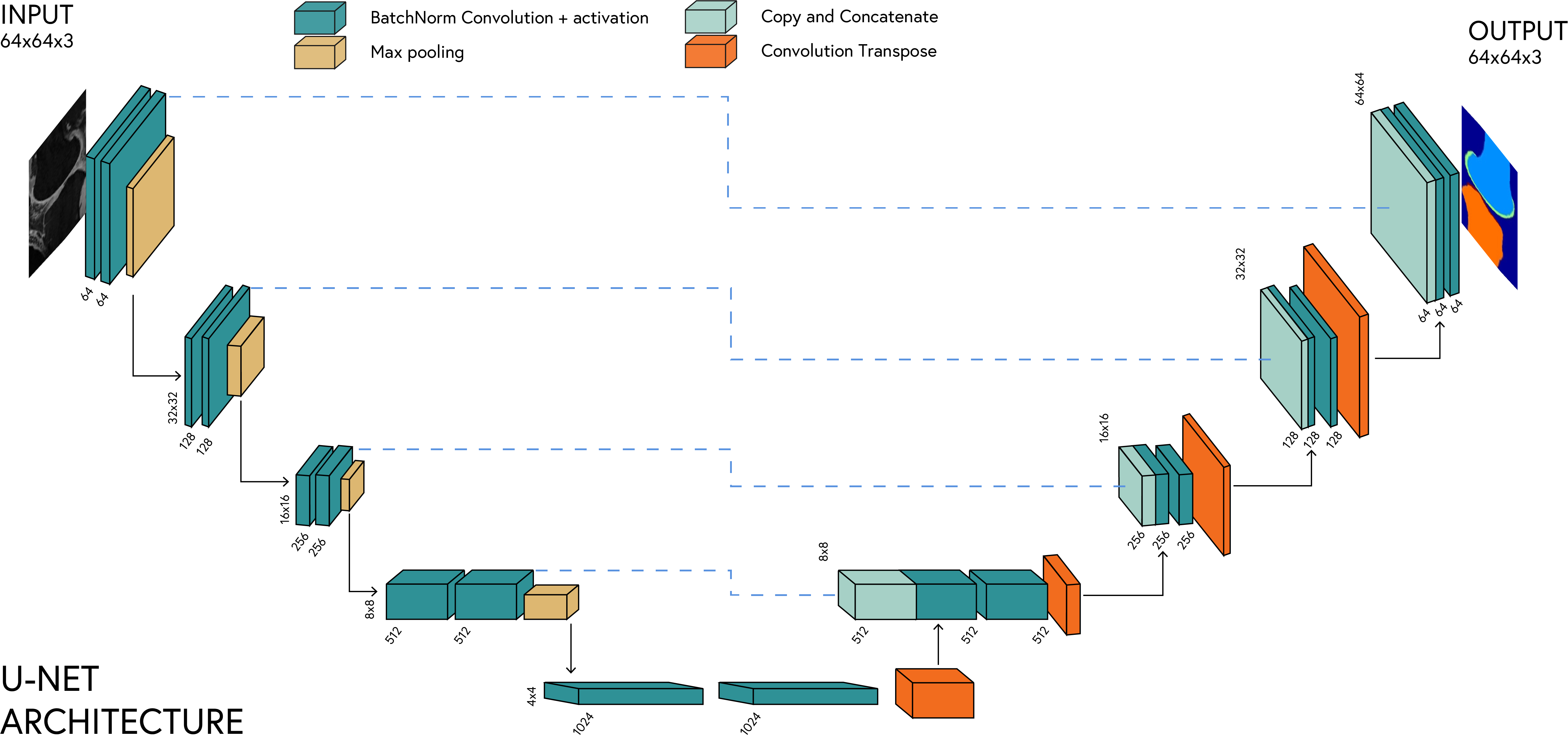
The U-Net architecture consists of two main parts: the encoder and the decoder, connected by skip connections. Each component plays a specific role:
| Component | Description | Purpose |
|---|---|---|
| Encoder (Contracting Path) | Series of convolutional and pooling layers | Captures context and semantic information |
| Decoder (Expanding Path) | Series of upsampling and convolutional layers | Enables precise localization |
| Skip Connections | Connect encoder layers to decoder layers | Preserve spatial information lost during downsampling |
| Bottleneck | Deepest layer connecting encoder and decoder | Captures the most complex features |
4.1 Transposed Convolution
For this architecture we are going to use a special type of convolutional layer that upsamples the input feature maps. This layer is called a transposed convolutional layer (also known as a deconvolutional layer). It is used to increase the spatial dimensions of the input feature maps, allowing the model to learn more complex features.
| Parameter | Description | Effect on Output |
|---|---|---|
| Kernel Size | Size of the filter | Determines area of influence |
| Stride | Step size of the filter | Controls amount of upsampling |
| Padding | Zero-padding added to input | Affects output size |
| Output Padding | Additional padding for output | Fine-tunes output dimensions |
The formula for calculating the output size of a transposed convolutional layer is:
\[\text{Output Size} = (\text{Input Size} - 1) \times \text{Stride} - 2 \times \text{Padding} + \text{Kernel Size} + \text{Output Padding}\]4.2 U-Net Implementation in PyTorch
We are going to implement the U-Net architecture using PyTorch. The implementation will consist of the following components:
| Component | Description |
|---|---|
DoubleConv |
A block that consists of two convolutional layers followed by batch normalization and ReLU activation. |
Down |
A block that consists of a max pooling layer followed by a DoubleConv block. |
Up |
A block that consists of a transposed convolutional layer followed by a DoubleConv block. |
UNet |
The main U-Net architecture that consists of the encoder and decoder blocks. |
# Exercise 6: Implementing the DoubleConv Block 🎯
# Implement:
# 1. Create a class called DoubleConv that inherits from nn.Module.
# 2. The constructor should take in the number of input channels and output channels.
# 3. Implement the forward method to apply two convolutional layers with ReLU activation and batch normalization.
# 4. Use kernel size 3 and padding 1 for both convolutional layers.
class DoubleConv(torch.nn.Module):
    def __init__(self, in_channels, out_channels):
        # Your code here: Initialize parent class
        super().__init__()
        # Your code here: Create a sequential module with two conv layers, each followed by batch norm and ReLU
        self.conv = torch.nn.Sequential(
            # Your code here: Conv2d with kernel_size=3, padding=1
            # Your code here: BatchNorm2d
            # Your code here: ReLU(inplace=True)
            # Your code here: Conv2d with kernel_size=3, padding=1
            # Your code here: BatchNorm2d
            # Your code here: ReLU(inplace=True)
        )

    def forward(self, x):
        # Your code here: Apply the sequential module to the input
        return # Your code here
# ✅ Check Exercise 6: DoubleConv Block Implementation
answer = {
'has_forward': hasattr(DoubleConv, 'forward'),
'has_two_conv_layers': str(DoubleConv(3, 64)).count('Conv2d') == 2,
'has_batch_norm': str(DoubleConv(3, 64)).count('BatchNorm2d') == 2,
'has_relu': str(DoubleConv(3, 64)).count('ReLU') == 2,
'uses_sequential': hasattr(DoubleConv(3, 64), 'conv') and isinstance(DoubleConv(3, 64).conv, torch.nn.Sequential)
}
checker.check_exercise(6, answer)# Exercise 7: Implementing the Down Block 🎯
# Implement:
# 1. Create a class called Down that inherits from nn.Module.
# 2. The constructor should take in the number of input channels and output channels.
# 3. Implement the forward method to apply a max pooling layer followed by the DoubleConv block.
# 4. Use a kernel size of 2 for the max pooling layer and stride of 2.
class Down(torch.nn.Module):
def __init__(self, in_channels, out_channels):
# Your code here: Initialize parent class
super().__init__()
# Your code here: Create a sequential module with MaxPool2d followed by DoubleConv
self.maxpool_conv = torch.nn.Sequential(
# Your code here: MaxPool2d with kernel_size=2
# Your code here: DoubleConv with in_channels and out_channels
)
def forward(self, x):
# Your code here: Apply the sequential module to the input
return # Your code here# ✅ Check Exercise 7: Down Block Implementation
answer = {
'has_forward': hasattr(Down, 'forward'),
'has_maxpool': str(Down(3, 64)).count('MaxPool2d') == 1,
'uses_doubleconv': str(Down(3, 64)).count('DoubleConv') == 1,
'uses_sequential': hasattr(Down(3, 64), 'maxpool_conv') and isinstance(Down(3, 64).maxpool_conv, torch.nn.Sequential)
}
checker.check_exercise(7, answer)# Exercise 8: Implementing the Up Block 🎯
# Implement:
# 1. Create a class called Up that inherits from nn.Module.
# 2. The constructor should take in the number of input channels and output channels.
# 3. Implement the forward method to apply a transposed convolution followed by the DoubleConv block.
# 4. Use a kernel size of 2 and stride of 2 for the transposed convolution.
# 5. Ensure to concatenate the feature maps from the encoder and decoder paths.
# 6. Handle the case where the sizes of the feature maps do not match by padding.
# 7. Use the torch.functional.pad function to pad the feature maps before concatenation.
class Up(torch.nn.Module):
def __init__(self, in_channels, out_channels):
# Your code here: Initialize parent class
super().__init__()
# Your code here: Create a transposed convolution with in_channels, in_channels//2
self.up = # Your code here
# Your code here: Create a DoubleConv with in_channels and out_channels
self.conv = # Your code here
def forward(self, x1, x2):
# Your code here: Apply the transposed convolution to x1
x1 = # Your code here
# Your code here: Calculate padding if needed to match dimensions
diffY = # Your code here
diffX = # Your code here
# Your code here: Pad x1 to match x2's dimensions
x1 = # Your code here
# Your code here: Concatenate x1 and x2 along the channel dimension
x = # Your code here
# Your code here: Apply the DoubleConv to the concatenated tensor
return # Your code here# ✅ Check Exercise 8: Up Block Implementation
answer = {
'has_forward': hasattr(Up, 'forward'),
'has_transpose_conv': hasattr(Up(64, 32), 'up') and isinstance(Up(64, 32).up, torch.nn.ConvTranspose2d),
'uses_doubleconv': hasattr(Up(64, 32), 'conv') and isinstance(Up(64, 32).conv, DoubleConv),
'handles_size_mismatch': 'diffY' in str(inspect.getsource(Up.forward)),
'uses_concat': 'torch.cat' in str(inspect.getsource(Up.forward))
}
checker.check_exercise(8, answer)# Exercise 9: Implementing the UNet Model 🎯
# Implement:
# 1. Create a class called UNet that inherits from nn.Module.
# 2. The constructor should take in the number of input channels and output channels.
# 3. Implement the forward method to define the architecture of the UNet model.
# 4. Use the DoubleConv, Down, and Up classes to build the encoder and decoder paths.
# 5. Ensure to include skip connections between the encoder and decoder paths.
# 6. Use a final convolutional layer to produce the output.
# 7. Use a kernel size of 1 for the final convolutional layer.
# 8. Apply a sigmoid activation function to the output layer.
class UNet(torch.nn.Module):
def __init__(self, in_channels=3, out_channels=1):
# Your code here: Initialize parent class
super().__init__()
# Initial convolution
# Your code here: Create a DoubleConv with in_channels and 64 output channels
self.inc = # Your code here
# Encoder path
# Your code here: Create Down modules with increasing channel depths
self.down1 = # Your code here: 64 -> 128
self.down2 = # Your code here: 128 -> 256
self.down3 = # Your code here: 256 -> 512
self.down4 = # Your code here: 512 -> 1024
# Decoder path
# Your code here: Create Up modules with decreasing channel depths
self.up1 = # Your code here: 1024 -> 512
self.up2 = # Your code here: 512 -> 256
self.up3 = # Your code here: 256 -> 128
self.up4 = # Your code here: 128 -> 64
# Output layer
# Your code here: Create Conv2d with 64 input channels, out_channels output channels, and kernel_size=1
self.outc = # Your code here
def forward(self, x):
# Encoder
# Your code here: Apply inc to input
x1 = # Your code here
# Your code here: Apply down1 to x1
x2 = # Your code here
# Your code here: Apply down2 to x2
x3 = # Your code here
# Your code here: Apply down3 to x3
x4 = # Your code here
# Your code here: Apply down4 to x4
x5 = # Your code here
# Decoder with skip connections
# Your code here: Apply up1 to x5 and x4
x = # Your code here
# Your code here: Apply up2 to x and x3
x = # Your code here
# Your code here: Apply up3 to x and x2
x = # Your code here
# Your code here: Apply up4 to x and x1
x = # Your code here
# Output layer
# Your code here: Apply outc to x
output = # Your code here
# Your code here: Apply sigmoid activation
return # Your code here# ✅ Check Exercise 9: UNet Model Implementation
answer = {
'has_forward': hasattr(UNet, 'forward'),
'has_encoder_path': hasattr(UNet(3, 1), 'inc') and hasattr(UNet(3, 1), 'down1'),
'has_decoder_path': hasattr(UNet(3, 1), 'up1') and hasattr(UNet(3, 1), 'up4'),
'has_final_conv': hasattr(UNet(3, 1), 'outc') and isinstance(UNet(3, 1).outc, torch.nn.Conv2d),
'uses_sigmoid': 'sigmoid' in str(inspect.getsource(UNet.forward))
}
checker.check_exercise(9, answer)4.3 Segmentation Loss Functions
While we can use a simple loss function like binary cross-entropy for segmentation tasks since we are dealing with binary masks, it is often not sufficient. This is because the model may learn to predict the background class (0) more often than the foreground class (1), leading to poor performance on the actual segmentation task.
To address this, we are going to introduce a more sophisticated loss function called the Dice Loss. The Dice Loss is based on the Dice coefficient, which measures the overlap between two sets. It is defined as:
\[\text{Dice} = \frac{2 |X \cap Y|}{|X| + |Y|}\]Where:
- $X$ is the predicted segmentation mask
- $Y$ is the ground truth segmentation mask
- $X \cap Y$ is the number of pixels in the intersection of the predicted and ground truth masks
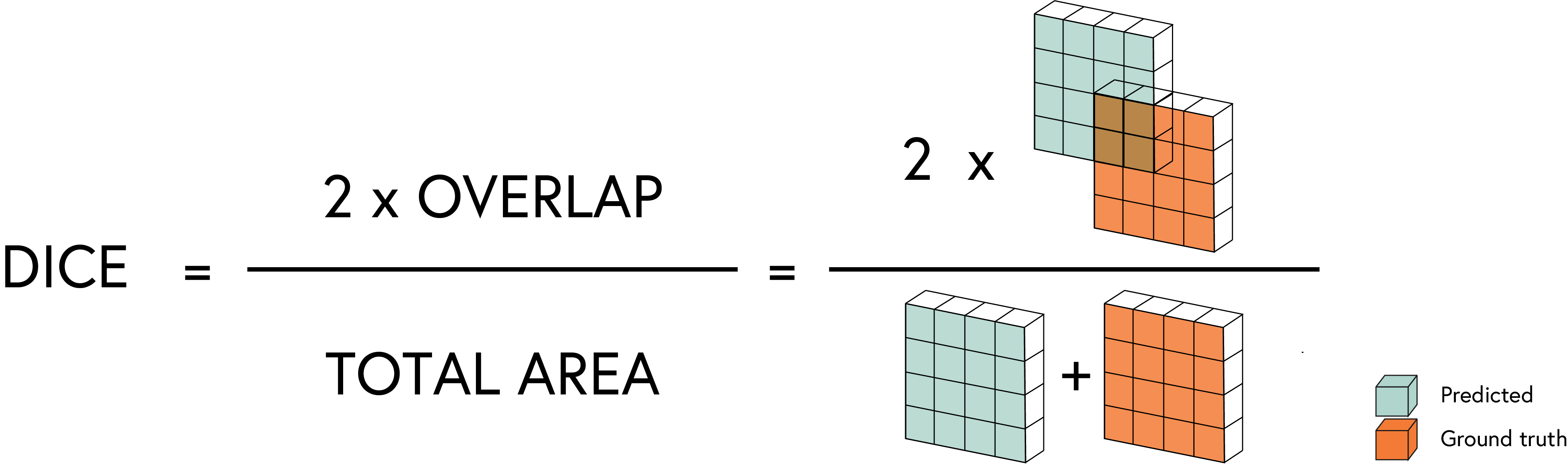
The Dice Loss is defined as:
\[\text{Dice Loss} = 1 - \text{Dice}\]4.3.1 Comparison of Segmentation Loss Functions
| Loss Function | Formula | Advantages | Disadvantages |
|---|---|---|---|
| Binary Cross-Entropy | $$ -\sum(y\log(\hat{y}) + (1-y)\log(1-\hat{y})) $$ | Easy to implement, works well for balanced classes | Poor performance with class imbalance |
| Dice Loss | $$ 1 - \frac{2\|X \cap Y\|}{\|X\| + \|Y\|} $$ | Handles class imbalance well, directly optimizes overlap | May get stuck in local minima |
| Focal Loss | $$ -\alpha(1-\hat{y})^\gamma y\log(\hat{y}) $$ | Focuses on hard examples, addresses class imbalance | Requires tuning of hyperparameters |
| IoU Loss | $$ 1 - \frac{\|X \cap Y\|}{\|X \cup Y\|} $$ | Directly optimizes intersection over union | Can be unstable for small regions |
| Combo Loss | $$ \alpha\cdot \text{BCE} + (1-\alpha)\cdot \text{Dice} $$ | Combines benefits of both BCE and Dice | Requires tuning of weighting parameter |
This loss function is particularly useful for imbalanced datasets, where the number of pixels in the foreground class is much smaller than the number of pixels in the background class. The Dice Loss penalizes the model more for misclassifying foreground pixels than background pixels, leading to better performance on the segmentation task.
# Exercise 10: Implementing the Dice Loss Function 🎯
# Implement:
# 1. Create a class called DiceLoss that inherits from nn.Module.
# 2. The constructor should take in a smoothing factor (default: 1.0).
# 3. Implement the forward method to calculate the Dice loss.
# 4. Ensure the inputs are properly shaped (flattened).

class DiceLoss(torch.nn.Module):
    def __init__(self, smooth=1.0):
        # Your code here: Initialize parent class
        super().__init__()
        # Your code here: Store the smoothing factor
        self.smooth = # Your code here

    def forward(self, y_pred, y_true):
        # Your code here: Flatten the prediction and target tensors to 1D
        y_pred = # Your code here
        # Your code here: Convert target tensor to float if needed
        y_true = # Your code here

        # Your code here: Calculate intersection (sum of element-wise multiplication)
        intersection = # Your code here
        # Your code here: Calculate union (sum of y_pred + sum of y_true)
        union = # Your code here

        # Your code here: Calculate Dice coefficient with smoothing factor
        dice = # Your code here: (2*intersection + smooth)/(union + smooth)

        # Your code here: Return loss (1 - dice), clamped between 0 and 1
        return # Your code here
# ✅ Check Exercise 10: Dice Loss Implementation
answer = {
'has_forward': hasattr(DiceLoss, 'forward'),
'handles_flattening': 'view(-1)' in str(inspect.getsource(DiceLoss.forward)),
'calculates_intersection': 'intersection' in str(inspect.getsource(DiceLoss.forward)),
'uses_smoothing': hasattr(DiceLoss(), 'smooth') and 'self.smooth' in str(inspect.getsource(DiceLoss.forward)),
'returns_1_minus_dice': '1 -' in str(inspect.getsource(DiceLoss.forward))
}
checker.check_exercise(10, answer)# Initialize the model, criterion, and optimizer
model = UNet(in_channels=3, out_channels=1).to(device)
criterion = DiceLoss()
optimiser = torch.optim.Adam(model.parameters(), lr=1e-3)
num_epochs = 2
# model = train_model(model, train_dl, valid_dl, criterion, optimizer, num_epochs)
model_v1 = utils.ml.train_model(
model=model,
criterion=criterion,
optimiser=optimiser,
train_loader=train_dl,
val_loader=valid_dl,
num_epochs=num_epochs,
early_stopping=True,
patience=3,
save_path= Path.cwd() / "my_models" / "se05_model_v1.pt",
plot_loss=True,
)# Show a batch of images and masks
test_ds = ISICDatasetAlbumentations(
image_dir=test_path,
mask_dir=test_mask_path,
transform=valid_img_ts
)
test_dl = DataLoader(test_ds, batch_size=16, shuffle=True)
utils.plotting.show_binary_segmentation_predictions(model_v1, test_dl, n_images=10, mean=mean, std=std)5. Transfer Learning with Pre-trained Models
In essence, the process of transfer learning involves taking a model that has been trained on a large dataset (the source domain) and adapting it to a new, smaller dataset (the target domain). This is done by reusing the learned features from the source model and fine-tuning them for the target task. The most common approach is to use the pre-trained model as a feature extractor, where the lower layers of the model are frozen and using a classifier head that is trained on the new dataset.
The process can be visualized as follows:
5.1 Pre-trained Models for Computer Vision
Several pre-trained models are available for computer vision tasks. Each has its own architecture, number of parameters, and performance characteristics:
| Model | Parameters | Input Size | Year | Top-1 Accuracy (ImageNet) | Architecture Highlights |
|---|---|---|---|---|---|
| ResNet | 11.7M - 60M | 224×224 | 2015 | 76.1% - 80.6% | Residual connections to combat vanishing gradients |
| VGG | 138M - 144M | 224×224 | 2014 | 71.3% - 75.6% | Simple architecture with small filters (3×3) |
| Inception | 6.8M - 54M | 299×299 | 2014 | 77.5% - 82.8% | Multi-scale processing with parallel paths |
| DenseNet | 8M - 44M | 224×224 | 2017 | 74.5% - 79.5% | Dense connections between layers for feature reuse |
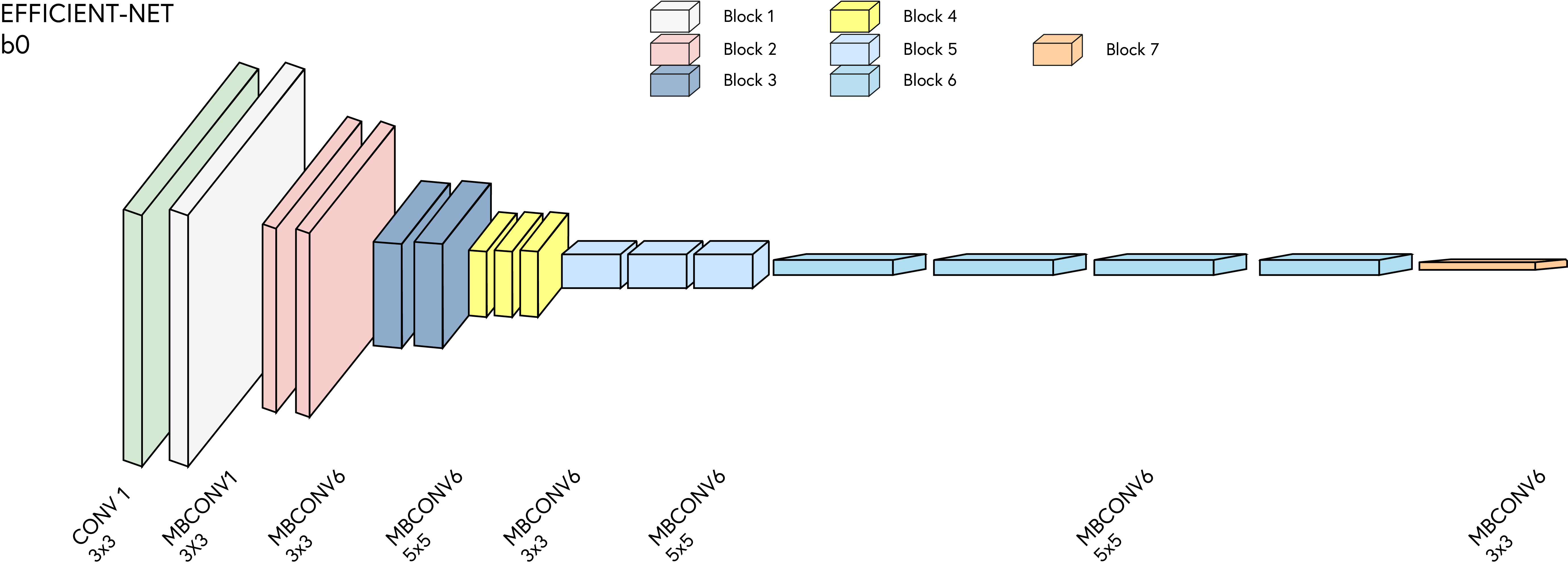
| EfficientNet | 5.3M - 66M | 224×224 - 600×600 | 2019 | 78.8% - 85.7% | Balanced scaling of depth, width, and resolution |
| MobileNet | 4.2M - 6.9M | 224×224 | 2017 | 70.6% - 75.2% | Designed for mobile devices with depthwise separable convolutions |
In this section, we are going to use a pre-trained model for the segmentation task. We are going to use an EfficientNet model that has been pre-trained on the ImageNet dataset. The EfficientNet model is a state-of-the-art convolutional neural network architecture that achieves high accuracy with fewer parameters compared to other architectures.
5.2 Transfer Learning Process
The typical transfer learning workflow consists of these steps:
| Step | Description | Technique |
|---|---|---|
| 1. Select Source Model | Choose a pre-trained model relevant to your target task | Select models trained on large datasets like ImageNet |
| 2. Feature Extraction | Use the pre-trained model as a fixed feature extractor | Freeze pre-trained layers, replace and retrain output layers |
| 3. Fine-tuning | Carefully adapt pre-trained weights to the new task | Gradually unfreeze layers, train with lower learning rates |
| 4. Model Adaptation | Modify architecture if needed for the target task | Add or remove layers as needed for the new domain |
5.3 Types of Transfer Learning
There are several approaches to implementing transfer learning:
| Approach | Description | Best Used When |
|---|---|---|
| Feature Extraction | Freeze pre-trained network, replace and retrain classifier | Target task is similar but dataset is small |
| Fine-Tuning | Retrain some or all layers of pre-trained network | Target task has sufficient data but benefits from pre-training |
| One-shot Learning | Learn from just one or very few examples | Extreme data scarcity |
| Domain Adaptation | Adapt to new data distribution without labels | Source and target domains have distribution shift |
| Multi-task Learning | Train model on multiple related tasks simultaneously | Related tasks can benefit from shared representations |
5.4 EfficientNet as an Encoder
The EfficientNet model is going to act as the encoder part of the U-Net architecture. We are going to replace the encoder part of the U-Net architecture with the EfficientNet model. The decoder part of the U-Net architecture will remain the same.
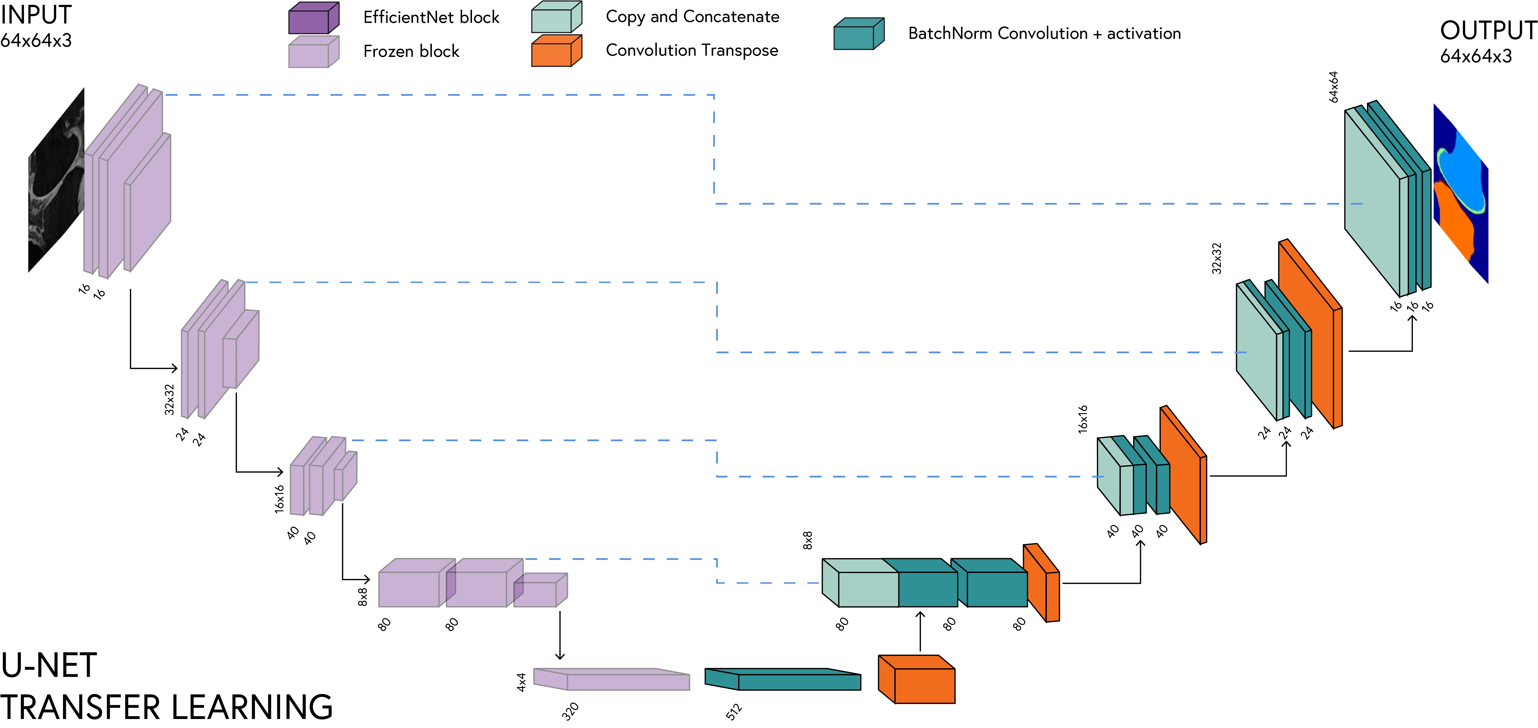
5.4.1 Transfer Learning Process for Segmentation
| Step | Description | Implementation Detail |
|---|---|---|
| 1. Extract Encoder | Use pre-trained EfficientNet as encoder | Remove classification head |
| 2. Add Decoder | Create U-Net style decoder | Transposed convolutions with skip connections |
| 3. Freeze Weights | Prevent pre-trained encoder from changing | Set requires_grad=False on encoder layers |
| 4. Train Decoder | Train only the decoder initially | Optimize only unfrozen parameters |
| 5. Fine-tune (Optional) | Gradually unfreeze encoder layers | Use lower learning rate for pre-trained layers |
from torchvision import models as tvm

efficientnet = tvm.efficientnet_b0(weights='IMAGENET1K_V1')
efficientnet = efficientnet.features  # Extract the feature extractor part
efficientnet = torch.nn.Sequential(*list(efficientnet.children())[:-1])  # Remove the classification head

for param in efficientnet.parameters():
    param.requires_grad = False  # Freeze all layers
# Exercise 11: Implementing U-Net with EfficientNet Encoder 🎯
# Implement:
# 1. Create a new Up class called SmartUp that inherits from nn.Module.
# 2. The constructor should take in the number of input channels, skip channels, and output channels.
# 3. Implement the forward method to apply a transposed convolution followed by the DoubleConv block.
# 4. Ensure to concatenate the feature maps from the encoder and decoder paths.
# 5. Handle the case where the sizes of the feature maps do not match by interpolation.
# 6. Use the torch.nn.functional.interpolate function to resize the feature maps before concatenation.
# 7. Use the torchvision.models.efficientnet_b0 model as the encoder.
# 8. Extract the feature layers from the EfficientNet model and use them in the UNet architecture.
# 9. Freeze the encoder layers to preserve the pretrained weights.
# 10. Use the DoubleConv block for the center bottleneck and decoder path.
# 11. Ensure to include skip connections between the encoder and decoder paths.
# 12. Use a final convolutional layer to produce the output.
# 13. Apply a sigmoid activation function to the output layer.

import torchvision.models as tvm

class SmartUp(torch.nn.Module):
    def __init__(self, in_channels, skip_channels, out_channels):
        # Your code here: Initialize parent class
        super(SmartUp, self).__init__()
        # Your code here: Create a transposed convolution
        self.up = # Your code here: ConvTranspose2d with in_channels, skip_channels, kernel_size=2, stride=2
        # Your code here: Create a DoubleConv with skip_channels*2 (for concatenation) and out_channels
        self.conv = # Your code here

    def forward(self, x1, x2):
        # Your code here: Apply transposed convolution to x1
        x1 = # Your code here

        # Your code here: Handle size mismatches with interpolation
        if x1.size()[2:] != x2.size()[2:]:
            # Your code here: Use nn.functional.interpolate to resize x1 to match x2's size
            x1 = # Your code here

        # Your code here: Concatenate the skip connection
        x = # Your code here
        # Your code here: Apply the convolutional block
        return # Your code here

class UNetEfficient(torch.nn.Module):
    def __init__(self, in_channels=3, out_channels=1):
        # Your code here: Initialize parent class
        super(UNetEfficient, self).__init__()

        # Your code here: Load pretrained EfficientNet
        efficient_net = # Your code here: tvm.efficientnet_b0 with weights='DEFAULT'

        # Your code here: Extract feature layers from EfficientNet - using UNet nomenclature
        # Extract the first two layers as the initial block
        self.inc = # Your code here
        # Extract the MBConv blocks as the down stages
        self.down1 = # Your code here: MBConv block 2
        self.down2 = # Your code here: MBConv block 3
        self.down3 = # Your code here: MBConv block 4
        self.down4 = # Your code here: MBConv blocks 5,6,7

        # Your code here: Freeze encoder layers to preserve pretrained weights
        encoders = [self.inc, self.down1, self.down2, self.down3, self.down4]
        for encoder in encoders:
            # Your code here: Loop through each parameter and set requires_grad to False
            # Your code here

        # Your code here: Get the output channels from each encoder stage
        enc1_channels = 16     # Initial block outputs 16 channels
        enc2_channels = 24     # MBConv block 2 outputs 24 channels
        enc3_channels = 40     # MBConv block 3 outputs 40 channels
        enc4_channels = 80     # MBConv block 4 outputs 80 channels
        enc5_channels = 320    # Last MBConv block outputs 320 channels

        # Your code here: Center bottleneck (using DoubleConv)
        self.center = # Your code here

        # Your code here: Upsampling path with SmartUp blocks
        self.up1 = # Your code here: SmartUp with 512, enc4_channels, enc4_channels
        self.up2 = # Your code here: SmartUp with enc4_channels, enc3_channels, enc3_channels
        self.up3 = # Your code here: SmartUp with enc3_channels, enc2_channels, enc2_channels
        self.up4 = # Your code here: SmartUp with enc2_channels, enc1_channels, enc1_channels

        # Your code here: Final output layer
        self.outc = # Your code here: Conv2d with enc1_channels, out_channels, kernel_size=1

    def forward(self, x):
        # Your code here: Save input size for later resizing if needed
        input_size = x.size()[2:]

        # Your code here: Encoder path with EfficientNet
        x1 = # Your code here: Apply inc to x
        x2 = # Your code here: Apply down1 to x1
        x3 = # Your code here: Apply down2 to x2
        x4 = # Your code here: Apply down3 to x3
        x5 = # Your code here: Apply down4 to x4

        # Your code here: Center processing
        x = # Your code here: Apply center to x5

        # Your code here: Decoder path with skip connections
        x = # Your code here: Apply up1 to x and x4
        x = # Your code here: Apply up2 to x and x3
        x = # Your code here: Apply up3 to x and x2
        x = # Your code here: Apply up4 to x and x1

        # Your code here: Final output layer
        output = # Your code here: Apply outc to x

        # Your code here: Resize to match original input dimensions if needed
        if output.size()[2:] != input_size:
            # Your code here: Use interpolate to resize output
            output = # Your code here

        # Your code here: Apply sigmoid activation and return
        return # Your code here
# Initialize the EfficientNet UNet model
model_efficient = UNetEfficient(in_channels=3, out_channels=1).to(device)
criterion_efficient = DiceLoss()
optimizer_efficient = torch.optim.Adam(filter(lambda p: p.requires_grad, model_efficient.parameters()), lr=1e-3)
num_epochs = 5
model_efficient = utils.ml.train_model(
model=model_efficient,
criterion=criterion_efficient,
optimiser=optimizer_efficient,
train_loader=train_dl,
val_loader=valid_dl,
num_epochs=num_epochs,
early_stopping=True,
patience=3,
save_path= Path.cwd() / "my_models" / "se05_model_v2.pt",
plot_loss=True,
)# Visualize predictions with EfficientNet UNet
utils.plotting.compare_binary_segmentation_models(
model_v1, model_efficient, test_dl, n_images=10, mean=mean, std=std)5.5 Advantages of Transfer Learning
Transfer learning is particularly effective in computer vision and natural language processing (NLP) tasks, where large pre-trained models are available. The key advantages of transfer learning include:
| Advantage | Description | Impact |
|---|---|---|
| Reduced Training Time | Start with pre-learned features instead of random weights | Training can be 5-10x faster than from scratch |
| Less Training Data | Leverage knowledge from the source domain | Can work with hundreds vs. thousands of examples |
| Better Performance | Often achieves higher accuracy than training from scratch | Especially beneficial with limited target data |
| Faster Convergence | Models typically reach optimal performance in fewer epochs | Reduces computational costs of model development |
| Lower Computational Cost | Requires fewer resources for training | Makes deep learning accessible with limited hardware |
| Knowledge Retention | Preserves useful features learned from large datasets | Captures generalizable representations across domains |
# Quiz on Transfer Learning Concepts
print("\n🧠 Quiz 2: Feature extraction vs. Fine Tuning")
quizzer.run_quiz(2)

print("\n🧠 Quiz 3: Selecting Pre-trained models")
quizzer.run_quiz(3)

print("\n🧠 Quiz 4: Transfer Learning Techniques")
quizzer.run_quiz(4)

print("\n🧠 Quiz 5: Transfer Learning Learning Rate Selection")
quizzer.run_quiz(5)